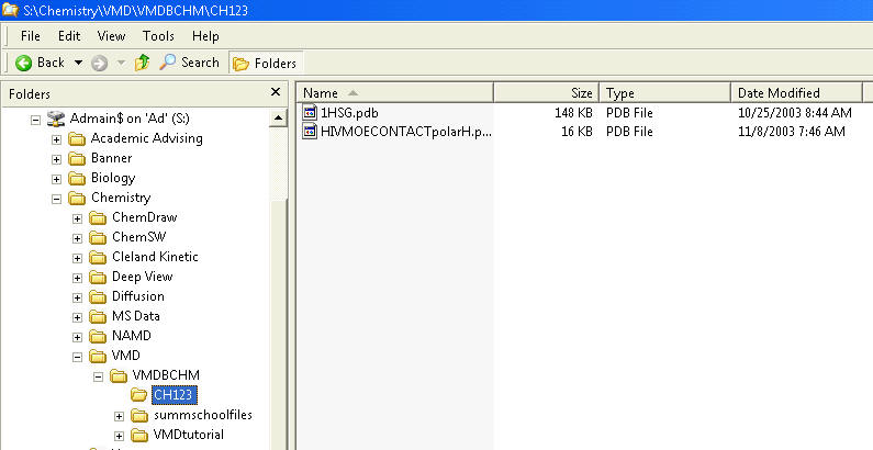
Select the drop down in the Look in: line. Then select Admain$ on 'Ad' (S:). The 1HSG.pdb file is located in the S:\Chemistry\VMD\VMDBCHM\CH123. Keep clicking until you get there, then select the file.
Chemistry and Medicine
Last update: 09/16/2008
Part 1: Structure makes a difference!
Some small molecules: water and ethanol
Part 2: Intermolecular Forces (IMFs) - from water to proteins
Hydrogen bonds - H bond: Water Jmol | liquid to solid transition Jmol
To bury or not. That is the question. A micelle
A typical protein: Triose Phosphate Isomerase
An alpha helix with H bonds
To bury or not. That is the question. A protein
A complex of two proteins: Thrombin and Hirudin
Part 3: HIV Protease: an Enzyme at Work - Video
Part 4: Molecular Modeling of the HIV Protease/Inhibitor Complex
In this exercise, you will study the structures of HIV protease and an inhibitor which binds to the protease. You will use a powerful molecular modeling program called VMD, which was developed at the University Illinois (Champaign/Urbana). For more information, see the website below
OpeningVMD
On a networked PC, select Start, All Programs, Academic Software, Chemistry, VMD 1.8.6. Three windows will open for you.
Our first step is to load our molecule. A pdb file,
1HSG.pdb, that contains the atom coordinates of HIV protease and an inhibitor is provided with the tutorial.Select the drop down in the Look in: line. Then select Admain$ on 'Ad' (S:). The 1HSG.pdb file is located in the S:\Chemistry\VMD\VMDBCHM\CH123. Keep clicking until you get there, then select the file.
Note that when you select the file, you will be
back in the Molecule File Browser window. In order to actually load the file
you have to press Load (d). Do not forget to do this!
 |
Now, HIV protease is shown in your screen in the OpenGL Display window. You may
close the Molecule File Browser window at any time. You will see
many red dots around the protein. These represent the oxygen of water
molecules that co-crystallized with the protein that was used to determine the
x-ray structure.
In order to see the 3D structure of our protein we will use the mouse and its multiple modes.
 |
 |
It should be noted that the previous actions performed with the mouse do not change the actual coordinates of the molecule atoms.
Another useful option is the Mouse
![]() Center
menu item. It allows you to specify the point around which rotations are done.
Center
menu item. It allows you to specify the point around which rotations are done.
VMD can display your molecule using a wide variety of drawing styles. Here,
we will explore those that can help you to identify different structures in the
protein.
 |
The previous representations allows you to see the micromolecular details of
your protein. However, more general structural properties can be seen by using
more abstract drawing methods.
The last drawing method we will explore here is called Cartoon. It
gives a simplified representation of a protein based in its secondary structure.
Helices are drawn as cylinders,
b
sheets as solid
ribbons and all other structures as a tube. This is probably the most popular
drawing method to view the overall architecture of a protein.
Let's look at different independent (and interesting) parts of our molecule.
Combinations of Boolean operators can also be used when writing a selection. The review below is from Wikipedia

"Venn diagram showing the intersection of sets "A AND B" (in violet/dark shading), the union of sets "A OR B" (all the colored/shaded regions), and the exclusive OR case "set A XOR B" (all the colored regions except the violet/only the lightly shaded regions). The "universe" is represented by all the area within the rectangular frame." AND limits the search while OR broadens it.
 |
The button Create Rep Fig
7(a) in the Graphical Representations window allows you to create multiple
representations and therefore have a mixture of different selections with
different styles and colors, all displayed at the same time.
 |
| To Display | Drawing Style | Coloring Method | Selection |
| c. Protein without water | Cartoon | Structure | protein |
| d. Protein Surface w/o water | Surface | Pos | protein |
| e. inhibitor alone | VDW - van der Waals | Molecule | (not protein) and (not water) |
| f. Protein and inhibitor | CPK | Name | all and (not water) |
Double click on the representations to toggle them off and on. Display just the Protein Surface (d) and the Inhibitor Alone (e). Toggle (e) on and off to see how the inhibitor fits snuggly into a cavity or "active" site in the protein. Likewise click display (c) and (e) alone. Again toggle on and off the inhibitor (e). Experiment with other options.
The complex you have seen above, no matter how you render it, is still quite complicated. We have used a program called MOE to create a file (HIVMOECONTACTpolarH.pdb) that shows only the inhibitor and the amino acids around it that make contacts. Load the file now.
Select the drop down in the Look in: line. Then select Admain$ on 'Ad' (S:). The HIVMOECONTACTpolarH.pdb file is located in the S:\Chemistry\VMD\VMDBCHM\CH123. Keep clicking until you get there, then select the HIVMOECONTACTpolarH.pdb fil
What properties must the inhibitor and binding pocket of the enzyme have in common to allow inhibitor binding? You discussed these earlier today and you will cover them more in depth in General Chemistry II (Chapter 10, Section 10.2). In essence there are intermolecular forces - forces between molecules that are distinguished from covalent bonds within a molecule) that allow reversible binding. In general, there are 3 types of intermolecular forces between the inhibitor and protease (the two different molecules) that may be involved here:
These same types of interactions allow binding of the inhibitor to HIV protease. Their binding surfaces are complementary. The list below shows the contacts between HIV protease and the inhibitor. Try to identify them in the active site file you just loaded.
Important Note: The first pdb file you loaded did not contain H atoms, since they are too small to be detect when the x-ray structure of the molecules was determined. In the second pdb file showing the active site, "polar" H atoms have been added to the protein and inhibitor by another software program called MOE. The chart below shows the H bonds occurring between N and O atoms, not between Hs on N and O atoms and N and O atoms. In the cases listed, a H atom is assumed to be linked by a covalent bond to one of the listed O or N atoms.
In the cells below, listings for the amino acids have the 3 letter name and number of the amino acid with the next letter representing the atom (O is oxygen, etc). For the inhibitor, MK1902 is the name of the inhibitor and the next letter stands of the atom followed by the number of that atom in the inhibitor.
|
Atom number |
Type contact |
Protease chain |
Amino acid(#), atom |
Atom on inhibitor |
|
23 |
H-BOND |
A |
ASP25.OD1 |
MK1902.O2 |
|
37 |
H-BOND |
B |
ASP25.OD1 |
MK1902.O2 |
|
38 |
H-BOND |
B |
GLY27.O |
MK1902.N4 |
|
39 |
H-BOND |
B |
ASP29.OD2 |
MK1902.O4 |
|
101 |
HYDROPHOBIC |
A |
LEU23.CD2 |
MK1902.C16 |
|
102 |
HYDROPHOBIC |
A |
VAL32.CG2 |
MK1902.C6 |
|
103 |
HYDROPHOBIC |
A |
ILE47.CD1 |
MK1902.C7 |
|
104 |
HYDROPHOBIC |
A |
ILE50.CG1 |
MK1902.C29 |
|
105 |
HYDROPHOBIC |
A |
VAL82.CG1 |
MK1902.C20 |
|
106 |
HYDROPHOBIC |
A |
ILE84.CD1 |
MK1902.C14 |
|
148 |
HYDROPHOBIC |
B |
VAL32.CG2 |
MK1902.C27 |
|
149 |
HYDROPHOBIC |
B |
ILE47.CD1 |
MK1902.C27 |
|
150 |
HYDROPHOBIC |
B |
ILE50.CG1 |
MK1902.C7 |
|
151 |
HYDROPHOBIC |
B |
ILE84.CD1 |
MK1902.C28 |
You can visualize the H bonds in VMD by:
Now create a new representation to change the rendering of the inhibitor to better identify nonpolar:nonpolar (hydrophobic) interactions
Hope you found this evening interesting and applicable to your interests.
Submitted Images from Fall 2008