Determination of Mechanism in Chemistry
Mathematical Tools in Kinetics
MK3. Experimental Determination of the Rate Law
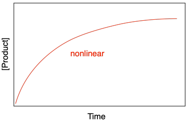
We have already looked at different forms of the rate law that researchers might use in different situations. Let's look at just a few of the things they might do as they are monitoring the progress of a reaction in the lab. One of the slightly complicated things about kinetics is the fact that we are looking at a relationship between concentration and time, a relationship that is nonlinear. If we look at product formation, product concentration grows quickly at first but then slows down.
Figure MK3.1 Product formation slowing down over time.
Of course, we know that happens because the reactant is getting consumed as the reaction progresses. As the reactant gets consumed, less of it is available to be converted into product, so the rate slows down.
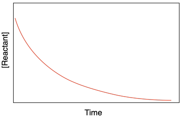
Figure MK3.2 Consumption of reactants slowing down over time.
Historically, interpreting nonlinear data is something people have tried to avoid. It's much easier to interpret simple, linear relationships, because we learn how to do that in grade school. We can all determine slopes and y intercepts fairly easily once someone has shown us how. Partly for that reason, there is a prevalent approach in kinetics called the "method of initial rates" that deliberately ignores most of the data in that graph and focuses on the very beginning.

Figure MK3.3 Approximation of the initial rate as a straight line.
Notice that at the very beginning of the graph, before the reactant concentration has changed much, the line hasn't really started to curve much. It stays pretty linear. In fact, we could take a snippet of the curve from any short segment along the plot and it would be fairly linear, provided the reactant didn't change very much over that portion of the data. However, the slope of the line at that point would change, depending upon how much reactant was left. At each of these points, the slope is equal to the rate of the reaction.
Rate = d[Product]/dt = Δ[Product]/Δt = slope
or d[Product]/dt = -d[Reactant]/dt = -Δ[Reactant]/Δt = - slope
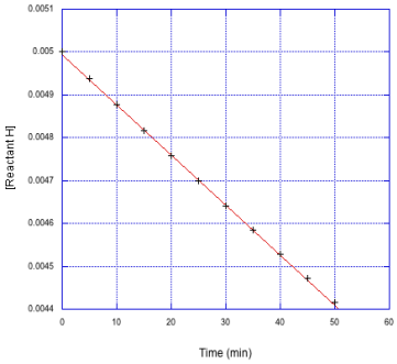
Since we know for sure what the reactant concentration is at the beginning, it makes sense to focus on that part. Let's take a look at how we might use some initial rate data. Here is a plot of data points for concentration measured over the first several minutes of a reaction. Depending on the speed of the reaction, this might be better represented as the first several seconds or the first several hours. The key point is that the concentration has hardly dropped during this time; for this approach to work, the change should be less than 10%.
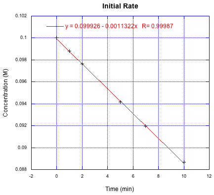
Figure MK3.4 A line of best fit through initial rate data.
If you look closely, you'll see that they went a little too far. Going to 10% completion would mean following the reaction until the concentration dropped from the initial 0.10 M to 0.09 M. Notice the last data point is a little above the line; that could just reflect regular experimental error, or it could be because we are looking at a broad enough slice of time that we are starting to see the curvature. (This is just fabricated data, so there's no one to blame for this mistake.)
To analyze the data, they would simply take the slope of the line and report that as the rate at initial concentration of reactant = 0.10 M. The linear regression has already done that for them, so the initial rate = 1.13 x 10⁻³ mol L-1 min-1.
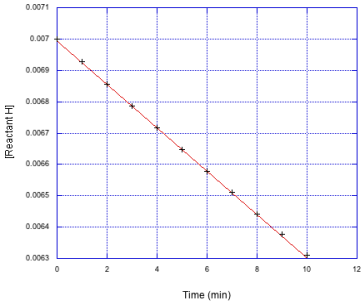
Problem MK3.1.
Determine the initial rate in each of the following cases.
a)
b)
c)
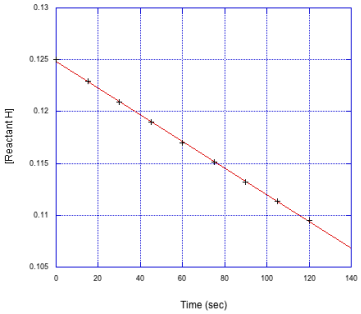
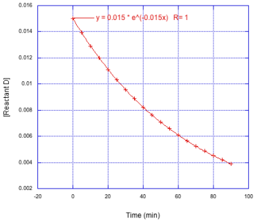
For comparison, we'll look at a full data set below. The data we saw before is scrunched into the top left hand corner of the graph. The reaction gets slower over time, and is hardly changing over the last two data points.
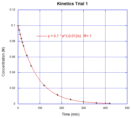
Figure MK3.5 The previous data set, extended over sevral half-lives.
Rather than fitting to a straight line, this graph has been fit to a linear regression for exponential decay. We've made the assumption that the reaction is first order in the reactant being monitored. In that case, the integrated rate law is logarithmic.
ln([Reactant]/[Reactant]0) = -kt
[Reactant]/[Reactant]0 = e-kt
[Reactant] = [Reactant]0 e-kt
So the pre-exponential factor is just the initial concentration and the fitted parameter in the exponent is the rate constant. In order to get a very good fit to the data, researcher will usually follow the reaction out to 3-5 half lives. They might stop at only three half-lives for convenience - five is getting to be a long time - or if there are competing processes that start to interfere with the data at longer times (maybe thermal decomposition if the reaction requires heating).
half life = t1/2 = 0.693/k
in this case, t1/2 = 0.693 / 1.2 x 10⁻² min-1 = 58 minutes
For visual confirmation, we can see that the concentration of reactant has dropped to about half after the first hour. The researchers have followed this reaction to about seven half lives, so they probably could have gone home sooner.
Problem MK3.2.
Determine the the number of half lives monitored in each of the following cases.
a)
b)
c)
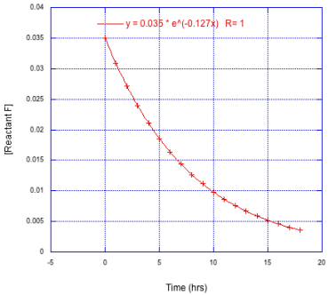
Having fit the entire course of the reaction to an exponential decay, we have been able to demonstrate that the reaction is first order in the reactant whose concentration we monitored. Otherwise, the curve would not have fit the data points very well. That's one of the advantages of analyzing the full data set with a nonlinear fit: we get an immediate rate constant as well as confirmation of first order behaviour.
What about if we were using the initial rates method? At low conversion, the plot should be linear no matter what, because the reactant concentration hasn't changed enough to severely impact the rate (unless the reaction is ninth order in that reactant or something like that; but even second order in one reactant is a relatively rare event). So how do we confirm the order?
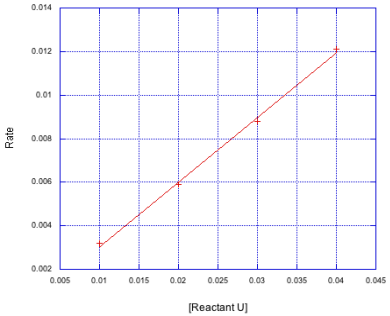
The approach is to run a few different initial rates experiments using different starting concentrations of reactant. If we take the slopes from each of those linear plots and compare them to the starting concentrations, a straight line relationship indicates first order. Furthermore, now we can get the rate constant, because the slope of this line is k.

Figure MK3.6 Plot of rate vs. initial concentration of a reactant.
Problem MK3.3.
Determine the rate constant in each of the following cases.
a)
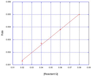
b)
c)
Frequently this constant is referred to as kobs, for the observed rate constant. It might not be the same as the true rate constant because there may be other reactant or catalyst concentrations that we know factor into things or that we still need to investigate. For example, in a catalyzed reaction, we might hold the catalyst concentration constant for these studies, having already extablished that the reaction is first order in catalyst. In that case, kobs = k[cat].
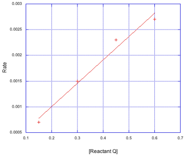
What if the order in some reactant turns out to be some number other than one? If it's zero order, of course that just means the rate is independent of the thing we decided to study, and the Rate vs. Concentration graph yields a horizontal line.
If it's higher order, the plot of rate vs. reactant wouldn't be linear. In such cases, it's common to make a log plot of the data. If that plot yields a linear relationship, it suggests a power law, in which the concentration is raised to an exponent.
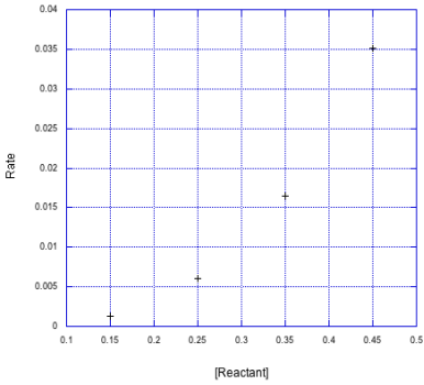
Figure MK3.7 A nonlinear plot of rate vs reactant concentration.
Let's see how that looks when the rate is plotted on a log scale.
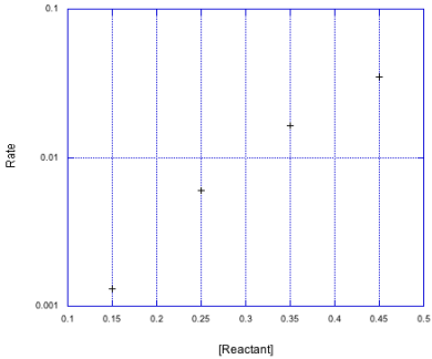
Figure MK3.8 The previous data set plotted with a logarithmic y-axis scale.
Sometimes it helps to compare a pair of data points using a logarithmic approach. If we take the ratio of rates, they should vary according to the rate law, which depends on the reactant concentration raised to some power.
rate1/rate2 = k[Reactant]1m / k[Reactant]2m = ([Reactant]1 / [Reactant]2)m
log(rate1/rate2) = m log([Reactant]1 / [Reactant]2)
m = log(rate1/rate2) / log([Reactant]1 / [Reactant]2)
Problem MK3.4.
Determine the order in each of the following cases.
a)
| [Reactant] | Rate |
| 0.0097 | 0.0944 |
| 0.0194 | 0.189 |
| 0.0291 | 0.283 |
b)
| [Reactant] | Rate |
| 0.25 | 0.101 |
| 0.50 | 0.806 |
| 0.75 | 2.72 |
c)
| [Reactant] | Rate |
| 1.50 | 0.000127 |
| 3.00 | 0.000508 |
| 4.50 | 0.00114 |
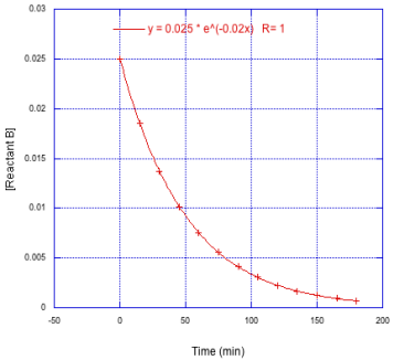
There are other complications that can arise in kinetics studies. One problem arises when the reaction rate depends on more than one reactant. That situation can lead to additional curvature in kinetic plots because more than one concentration is changing simultaneously. The common approach to dealing with this problem is to use "flooding" or "pseudo first order conditions". In this method, all of the reagents except one are held in vast excess, maybe ten times greater than a specific reagent of interest.
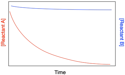
Figure MK3.9 Apparent curvature in rate data for Reactant B caused by changes in [Reactant A].
Under those conditions, the excess concentrations essentially remain constant. If they are constant, their values are absorbed into the rate constant, and the reaction depends only on the one reagent.
Rate = k[A][B]
but if [B] remains constant,
Rate = kobs[A]
where kobs = k[B]
Sometimes, a complementary approach is taken in which the concentration of interest is the one that is held in large excess. Because that relatively constant concentration is absorbed into the rate constant, running the reaction with three different levels of excess reagent yields three different values of kobs. A linear plot of kobs vs. concentration suggets a first order reaction.
Instrumental analysis greatly facilitates kinetic measurements, but there can be limitations to their use. For example, spectroscopic methods can be used to measure concentrations of reagents, but at some concentrations the instrumental signal may not respond proportionally to concentration. Researchers will often construct calibration curves to confirm the response of the instrument across the range of concentrations under study.
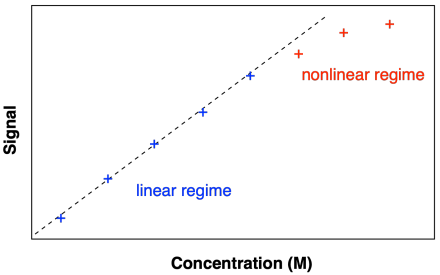
Figure MK3.10 Illustration of a calibration curve showing a linear relationship across a limited range of concentrations.
Even if we have a generally linear response, there can sometimes be drift in the instrumental signal over time that can interfere with the results. A common approach to that problem is to use an internal standard. That's a calibrated amount of a known compound with a known response under the instrumental method. If the response due to the compound of interest varies over time, so will the response due to the internal standard. The subject response can be standardized, for example by taking the ratio of the subject peak to the standard peak, to correct for fluctuations over time.
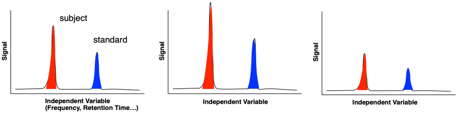
Figure MK3.11 An internal standard is used to correct for fluctuations in instrument signal over time.
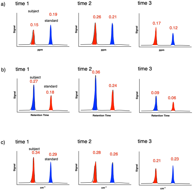
Problem MK3.5.
Determine whether the subject peak integration is increasing, decreasing, or staying constant in the following cases..
This site was written by Chris P. Schaller, Ph.D., College of Saint Benedict / Saint John's University (with contributions from other authors as noted). It is freely available for educational use.

Structure & Reactivity in Organic, Biological and Inorganic Chemistry by Chris Schaller is licensed under a Creative Commons Attribution-NonCommercial 3.0 Unported License.
Navigation: