CHAPTER 6 - TRANSPORT AND KINETICS

C: ENZYME INHIBITION

BIOCHEMISTRY - DR. JAKUBOWSKI

06/12/2014

C1.  Irreversible Covalent Inhibition

Given what you already know about protein structure, it should be easy to figure how to inhibit an enzyme. Since structure mediates function, anything that would significantly change the structure of an enzyme would inhibit the activity of the enzyme. Hence extremes of pH and high temperature, all of which can denature the enzyme, would inhibit the enzyme in a irreversible fashion, unless it could refold properly. Alternatively we could add a small molecule which interacts noncovalently with the enzyme to either change its conformation or directly prevent substrate binding. Finally, we could covalently modify certain side chains, that if they are essential to enzymatic activity, would irreversibly inhibit the enzyme.

We discussed previously the types of reagents that would chemically modify specific side chains that might be critical for enzymatic activity. For example, iodoacetamide might abolish enzyme activity if a Cys side chain is required for activity. These reagents will usually modify several side chains, however, and determining which is critical for binding or catalytic conversion of the substrate can be difficult. One way would be to protect the active site with a saturating quantities of a ligand which binds reversibly at the active site. Then the chemical modification can be performed at varying reaction times. The critical side chain would be protected from the chemical modification, but the extent of protection would depend on the Kd, concentration of the protecting ligand., and the length of the reaction.

more TBA

The rest of the chapter will deal with reversible, noncovalent inhibition

C2. Competitive Inhibition

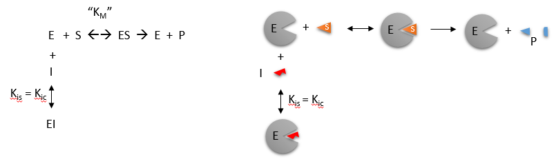
Reversible Competitive inhibition occurs when substrate (S) and inhibitor (I) both bind to the same site on the enzyme. In effect, they compete for the active site and bind in a mutually exclusive fashion. This is illustrated in the chemical equations and molecular cartoon below.

There is another type of inhibition that would give the same kinetic data.  If S and I bound to different sites, and S bound to E and produced a conformational change in E such that I could not bind (and vice versa), then the binding of S and I would be mutually exclusive. This is called allosteric competitive inhibition. Inhibition studies are usually done at several fixed and non-saturating concentrations of I and varying S concentrations.

The key kinetic parameters to understand are Vm and Km. Let us assume for ease of equation derivation that I binds reversibly, and with rapid equilibrium to E, with a dissociation constant Kis. The "s" in the subscript "is" indicates that the slope of the 1/v vs 1/S  Lineweaver-Burk plot changes while the y intercept stays constant.  Kis is also named K_ic where the subscript "c" stands for competitive inhibition constant.

A look at the top mechanism shows that even in the presence of I, as S increases to infinity, all E is converted to ES. That is, there is no free E to which I could bind. Now remember that Vm= kcatEo. Under these condition, ES = Eo; hence v = Vm.   Vm is not changed. However, the apparent Km, Kmapp, will change. We can use LaChatelier's principle to understand this. If I binds to E alone, and not ES, it will shift the equilibrium of E + S <==> ES to the left, which would have the affect of increasing the Km app (i.e. it would appear that the affinity of E and S has decreased.). The double reciprocal plot (Lineweaver Burk plot) offers a great way to visualize the inhibition. In the presence of I, Vm does not change, but Km appears to increase. Therefore, 1/Km, the x-intercept on the plot will get smaller, and closer to 0. Therefore the plots will consists of a series of lines, with the same y intercept (1/Vm), and the x intecepts (-1/Km) closer and closer to the 0 as I increases. These intersecting plots are the hallmark of competitive inhibition. 

Note that in the first three inhibition models discussed in this section, the Lineweaver-Burk plots are linear in the presence and absence of inhibitor.  This suggests that plots of v vs S in each case would be hyperbolic and conform to the usual form of the Michaelis Menton equation, each with potentially different apparent Vm and Km values.

An equation, shown in the figure above, can be derived which shows the effect of the competitive inhibitor on the velocity of the reaction. The only change is that the Km term is multiplied by the factor 1+I/Kis. Hence Kmapp = Km(1+I/Kis). This shows that the apparent Km does increase as we predicted. Kis is the inhibitor dissociation constant in which the inhibitor affects the slope of the double reciprocal plot. 

Wolfram Mathematica CDF Player - Competitive Inhibition v vs S (free plugin required)

4/6/14Wolfram Mathematica CDF Player - Competitive Inhibition - Lineweaver Burk(free plugin required)

If the data was plotted as vo vs log S, the plots would be sigmoidal, as we saw for plots of ML vs log L in Chapter 5B.   In the case of competitive inhibitor, the plot of  vo vs log S in the presence of different fixed concentrations of inhibitor would consist of a series of sigmoidal curves, each with the same Vm, but with different apparent Km values (where Kmapp = Km(1+I/Kis), progressively shifted to the right.   Enyzme kinetic data is rarely plotted this way, but simple binding data for the M + L < == > ML equilibrium, in the presence of different inhibitor concentrations is. 

Reconsider our discussion of the simple binding equilibrium, M + L <==> ML.  When we wished to know how much is bound, or the fractional saturation, as a function of the log L, we considered  three examples.

1. L = 0.01 Kd (i.e. L << Kd), which implies that Kd = 100L.  Then Y = L/[Kd+L] = L/[100L + L] ≈1/100.  This implies that irrespective of the actual [L], if L = 0.01 Kd, then Y ≈0.01. 
2. L = 100 Kd (i.e. L >> Kd), which implies that Kd = L/100.  Then Y = L/[Kd+L] = L/[(L/100) + L] = 100L/101L ≈ 1.  This implies that irrespective of the actual [L], if L = 100 Kd, then Y ≈1.
3. L = Kd, then Y = 0.5

These scenarios show that if L varies over 4 orders of magnitude (0.01Kd < Kd < 100Kd), or, in log terms, from
-2 + log Kd < log Kd  < 2 + log Kd),  irrespective of the magnitude of the Kd, that Y varies from approximately 0 - 1. 

In other words, Y varies from 0-1 when L varies from log Kd by +2.  Hence, plots of Y vs log L for a series of binding reactions of increasingly higher Kd (lower affinity) would reveal a series of identical sigmoidal curves shifted progressively to the right, as shown below. 

The same would be true of vo vs S in the presence of different concentration of a competitive inhibitor, for initial flux, Jo vs ligand outside, in the presence of a competitive inhibitor, or ML vs L (or Y vs L) in the presence of a competitive inhibitor.

Wolfram Mathematica CDF Player - Competitive Inhibition v vs logS (free plugin required)

In many ways plots of v0 vs lnS are easier to visually interpret than plots of v0 vs S .  As noted for simple binding plots, textbook illustrations of hyperbolas are often misdrawn, showing curves that level off too quickly as a function of [S] as compared to plots of  v0 vs lnS, in which it is easy to see if saturation has been achieved.  In addition, as the curves above show, multiple complete plots of v0 vs lnS at varying fixed inhibitor concentration or for variant enzyme forms (different isoforms, site-specific mutants) over a broad range of lnS can be made which facilitates comparisons of the experimental kinetics under these different conditions.  This is especially true if Km values differ widely. 

Now that you are more familiar with binding, flux, and enzyme kinetics curves, in the presence and absence of inhibitors, you should be able to apply the above analysis to inhibition curves where the binding, initial flux, or the initial velocity is plotted at varying competitive inhibitor concentration at different  fixed concentration nonsaturating concentrations of ligand or substrate. Consider the activity of an enzyme.  Lets say that at some reasonable concentration of substrate (not infinite), the enzyme is approximately 100% active. If a competitive inhibitor is added, the activity of the enzyme would drop until at saturating (infinite) I, no activity would remain.  Graphs showing this are shown below.

Figure:  Inhibition of Enzyme Activity - % Activity vs log [Inhibitor]

A special case of competitive inhibition: the specificity constant:  In the previous chapter, the specificity constant was defined as kcat/KM which we also described as the second order rate constant associated with the bimolecular reaction of E and S when S << KM.  It also describes how good an enzyme is in differentiating between different substrates.  If has enzyme encounters two substrates, one can be considered to be a competitive inhibitor of the other.  The following derivation shows that the ratio of initial velocities for two competing substrates at the same concentration is equal to the ratio of their kcat/KM values.

Java Applet: Competitive Inhibition I;   Competitive Inhibition II

C3.  Uncompetitive Inhibition

Reversible uncompetitive inhibition occurs when I binds only to ES and not free E. One can hypothesize that on binding S, a conformational change in E occurs which presents a binding site for I.  Inhibition occurs since ESI can not form product. It is a dead end complex which has only one fate, to return to ES. This is illustrated in the chemical equations and molecular cartoon below.

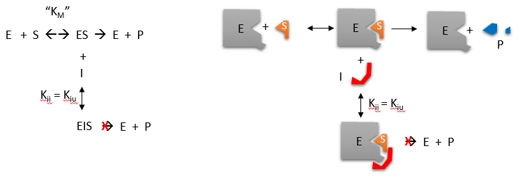
 Let us assume for ease of equation derivation that I binds reversibly to ES with a dissociation constant K_ii.  The second "i" in the subscript "ii" indicates that the intercept of the 1/v vs 1/S  Lineweaver-Burk plot changes while the slope stays constant.  Kii is also named K_iu, where the subscript "u" stands for the uncompetitive inhibition constant.

A look at the top mechanism shows that in the presence of I, as S increases to infinity, not all of E is converted to ES. That is, there is a finite amount of ESI, even at infinite S. Now remember that Vm = kcatEo if and only if all E is in the form ES . Under these conditions, the apparent Vm, Vmapp is less than the real Vm without inhibitor. In addition, the apparent Km, Kmapp, will change. We can use LaChatelier's principle to understand this. If I binds to ES alone, and not E, it will shift the equilibrium of E + S <==> ES to the right , which would have the affect of decreasing the Kmapp (i.e. it would appear that the affinity of E and S has increased.). The double reciprocal plot (Lineweaver Burk plot) offers a great way to visualize the inhibition. In the presence of I, both Vm and Km decrease. Therefore, -1/Km, the x-intercept on the plot, will get more negative, and 1/Vm will get more positive. It turns out that they change to the same extent. Therefore the plots will consist of a series of parallel lines, which is the hallmark of uncompetitive inhibition.

An equation, shown in the diagram above, can be derived which shows the effect of the uncompetitive inhibitor on the velocity of the reaction. The only change is that the S term in the denominator is multiplied by the factor 1+I/Kii. We would like to rearrange this equation to show how Km and Vm are affected by the inhibitor, not S, which obviously isn't. Rearranging the equation as shown above shows that Kmapp = Km/(1+I/Kii) and Vmapp = Vm/(1+I/Kii).   This shows that the apparent Km and Vm do decrease as we predicted. Kii is the inhibitor dissociation constant in which the inhibitor affects the intercept of the double reciprocal plot. Note that if I is zero, Km and Vm are unchanged.

Java Applet: Uncompetitive Inhibition

Wolfram Mathematica CDF Player - Uncompetitive Inhibition v vs S (free plugin required)

4/6/14Wolfram Mathematica CDF Player - Uncompetitive Inhibition - Lineweaver Burk(free plugin required)

C4. Noncompetitive and Mixed Inhibition

Reversible noncompetitive inhibition occurs when I binds to both E and ES. We will look at only the special case in which the dissociation constants of I for E and ES are the same. This is called noncompetiive inhibition. It is quite rare as it would be difficult to imagine a large inhibitor which inhibits the turnover of bound substrate having no effect on binding of S to E.  However covalent interaction of protons with both E and ES can lead to noncompetitive inhibition.   In the more general case, the Kd's are different, and the inhibition is called mixed. Since inhibition occurs, we will hypothesize that ESI can not form product. It is a dead end complex which has only one fate, to return to ES or EI. This is illustrated in the chemical equations and in the molecular cartoon below.

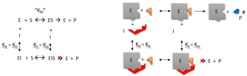
Let us assume for ease of equation derivation that I binds reversibly to E with a dissociation constant of Kis (as we denoted for competitive inhibition) and to ES with a dissociation constant Kii (as we noted for uncompetitive inhibition). Assume for noncompetitive inhibition that Kis = Kii. A look at the top mechanism shows that in the presence of I, as S increases to infinity, not all of E is converted to ES. That is, there is a finite amount of ESI, even at infinite S. Now remember that Vm = kcatEo if and only if all E is in the form ES . Under these conditions, the apparent Vm, Vmapp is less than the real Vm without inhibitor. In contrast, the  apparent Km, Kmapp, will not change since I binds to both E and ES with the same affinity, and hence will not perturb that equilibrium, as deduced from LaChatelier's principle. The double reciprocal plot (Lineweaver Burk plot) offers a great way to visualize the inhibition. In the presence of I, just Vm will decrease. Therefore, -1/Km, the x-intercept will stay the same, and 1/Vm will get more positive. Therefore the plots will consists of a series of lines intersecting on the x axis, which is the hallmark of noncompetitive inhibition. You should be able to figure out how the plots would appear if Kis is different from Kii (mixed inhibition).
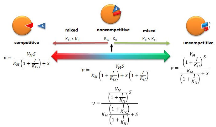
An equation, shown in the diagram above can be derived which shows the effect of the noncompetitive inhibitor on the velocity of the reaction. In the denominator, Km is multiplied by 1+I/Kis, and S by 1+I/Kii. We would like to rearrange this equation to show how Km and Vm are affected by the inhibitor, not S, which obviously isn't. Rearranging the equation as shown above shows that Kmapp = Km(1+I/Kis)/(1+I/Kii) = Km when Kis=Kii, and Vmapp = Vm/(1+I/Kii).  This shows that the Km is unchanged and Vm decreases as we predicted. The plot shows a series of lines intersecting on the x axis. Both the slope and the y intercept are changed, which are reflected in the names of the two dissociation constants, Kis and Kii. Note that if I is zero, Kmapp = Km and Vmapp = Vm.  Sometimes the Kis and Kii inhibition dissociations constants are referred to as Kc and Ku (competitive and uncompetitive inhibition dissociation constants.

Mixed (and non-)competitive inhibition (as shown by mechanism above) differ from competitive and uncompetiive inhibition in that the inhibitor binding is not simply a dead end reaction in which the inhibitor can only dissociate in a single reverse step.  In the above equilibrium, S can dissociate from ESI to form EI so the system may not be at equilibrium. With dead end steps, no flux of reactants occurs through the dead end complex so the equilibrium for the dead end step is not perturbed. 

Other mechanisms can commonly give mixed inhibition.  For example, the product released in a ping pong mechanism (discussed in the next chapter) can give mixed inhibition.

If P, acting as a product inhibitor, can bind to two different forms of the enzyme (E' and also E), it will act as an mixed inhibitor.

Java Applet:  Noncompetitive Inhibition

4/26/13Wolfram Mathematica CDF Player - Mixed Inhibition v vs S curves; Kis and Kii called Kc and Ku (start sliders at high values) (free plugin required)

4/26/13Wolfram Mathematica CDF Player - Mixed Inhibition v vs S curves (start sliders at high values) (free plugin required). Note where the inhibited and inhibited curves intersect at different values of Kis and Kii (in the graph termed Kc and Ku).

If you can apply LeChatilier's principle, you should be able to draw the Lineweaver-Burk plots for any scenario of inhibition or even the opposite case, enzyme activation!

Figure:  Summary of Reversible Enzyme Inhibition

C5.  Enzyme Inhibition in Vitro

The whole pharmaceutical industrial is devoted to finding drug molecules that affect biological processes.  Usually this means the development of small molecule inhibitors of target proteins, although recent work has expanded to development of inhibitory RNA molecules that affect DNA transcription and mRNA translation.  Using combinatorial synthetic techniques and computational modeling, it has gotten easier to develop small molecule inhibitors (especially competitive ones) that inhibit proteins in vitro using purified enzymes, substrates, and inhibitors in lab testing.  Assuming that the inhibitor could pass through the membrane and accumulate to a sufficient enough concentration, would it have the same inhibitory properties in the cell as in the test tube?  The answer turns out to be maybe.   Remember that a cell is tightly packed with a multitude of other small molecules and macromolecules.  In addition, the enzyme targeted for inhibition is most likely in part of a pathway of enzymes that feeds reactant into the enzyme and removes the product.  Hence the flux of substrate and product is controlled by the entire pathway and not just the single target enzyme although the product concentration of the target  enzyme  is determined by kinetic parameters for the enzyme and available substrate concentration. .

The conditions under which the enzymes are studied (in vitro) and operate (in vivo) are very different. 

• In vitro (in the lab), the enzyme is held at a constant concentration while the substrate is varied (i.e the substrate concentration is the independent variable).  The velocity is determined by the substrate concentration.  When inhibition is studied, the substrate is varied while the inhibitor is held constant at several different fixed concentrations. 

• In vivo (in the cell), the velocity might be held at a relatively fixed level with the substrate determined by the velocity.  To avoid a bottleneck in flux, substrate can't build up at the enzyme, so the enzyme processes it in a steady state fashion to produce product as determined by the Michael-Menten equation.

What happens when an inhibitor is added in vivo?  Let's assume that the enzyme is running at v = Vm/2.  We saw before for in vitro inhibition that it is sometimes difficult to differentiate competitive and uncompetiive inhibition (as evidenced from real, not hypothetical perfect double reciprocal plots).  How might in vivo inhibition plots look at constant velocity (for example v=Vm/2) when both I and S can vary and in which S for an enzyme in the middle of a pathway is determined by v?

The equations and graph below shows the ratio of S/Km vs I/Kix for inhibition at constant v, a condition encountered when an enzyme in a metabolic pathways is subject to flux controls imposed by the entire pathway.  The x axis reflects the relative amount of inhibitor compared to its inhibition constant.    Likewise the y axis reflects the relative amount of substrate compared to its Km.  The graph for in vivo competitive inhibition is linear, but it "blows up" for uncompetitive inhibition.

Figure:  Competitive and Uncompetitive Inhibition in vivo

Competitive Inhibition at Contant v		Uncompetitive Inhibition at Contant v

These graphs and associated equations are dramatically different from the very similar forms of inhibition equations and curves for in vitro inhibition at varying S and different fixed values of inhibitor.  Consider the uncompetitive graph and equation. In the absence of inhibitor, if S=Km, then Vm/v = 2 and, of course, the calculated value from the equation above of S/Km = 1. If I is allowed to increase to a value of Kii, again at constant v=Vm/2, then the right hand side goes to infinity. 

In a linked series of reaction, if the middle reaction is inhibited, the substrate for that enzyme builds, whether the inhibition is competitive or uncompetitive. With competitive inhibition, the substrate concentration can be raised to meet the requirements of the enzyme.  But as the above figure shows, this can't happen for uncompetitive inhibition since as more substrate accumulates, the reaction reaches a point where the steady state is lost.

Obviously, this limiting case can't be realistically reached but it does suggest that uncompetitive inhibitors would be more effective in vivo in controlling a metabolic pathway than competitive inhibitors.  Cornish-Bowden argues that purely uncompetitive inhibitors are rare in nature because of the degree of inhibition they can hypothetical produce (1986).  Likewise he suggests that medicinal chemists should synthesize uncompetitive inhibitors if their goal is to maximally inhibit a metabolic pathway under the kind of flux control described above.  Although it is more difficult to synthesis a purely uncompetitive inhibitor (as it can't be modeled after the structure of a natural ligand that bind to the active site and are competitive inhibitors, he notes synthesizing mixed (and noncompetitive) inhibitors whose Kii values are of reasonable size compared to their Kis values, would be one approach to try.

C6.  Agonist and Antagonist of Ligand Binding to Receptors - An Extension

The analysis of competitive, uncompetitive and noncompetitive inhibitors of enzymes can now be extended to understand how the activity of membrane receptors are affected by the binding of drugs.  When receptors bind their natural target ligands (hormones, neurotransmitters), a biological effect is elicited.  This usually involves a shape change in the receptor, a transmembrane protein, which activates intracellular activities.  The bound receptor usually does not directly express biological activity, but initiates a cascade of events which leads to expression of intracellular activity.  In some cases, however, the occupied receptor actually expresses biological activity itself.  For example, the bound receptor can acquire  enzymatic activity, or become an active ion channel. 

Drugs targeted to membrane receptors can have a variety of effects.  They may elicit the same biological effects as the natural ligand.  If so, they are called agonists.  Conversely they may inhibit the biological activity of the receptor.  If so they called antagonists

Agonist

An agonist is a mimetic of the natural ligand and produces a similar biological effect as the natural ligand when it binds to the receptor.  It binds at the same binding site, and leads, in the absence of the natural ligand, to either a full or partial response.  In the latter case, it is called a partial agonist.  The figure below shows the action of ligand, agonist, and partial agonist. 

There is another kind of agonist, given the bizarre name inverse agonist.  This term only makes sense when applied to a receptor that has a basal (or constitutive) activity in the absence of a bound ligand.  If either the natural ligand or an agonist binds to the receptor site, the basal activity is increased.  If however, an inverse agonists binds, the activity is decreased.   An example of an inverse agonist (which we will discuss later) is the binding of the drug Ro15-4513 to the GABA receptor, which also binds benzodiazepines such as valium.  When occupied by its natural ligand, GABA, the protein receptor is "activated" to become a channel allowing the inward flow of Cl- into a neural cell, inhibiting neuron activation.  Valium potentiates the effect of GABA, which is enhanced even further in the presence of ethanol.    Ro15-4513 binds to the benzodiazepine site, which leads to the opposite effect of valium, the inhibition of the receptor bound activity - a chloride channel. 

 Figure: Agonist and Partial Agonists

Antagonists

As there name implies, antagonist inhibit the effects of the natural ligand (hormone, neurotransmitter), agonist, partial agonist, and even inverse agonists.  We can think of them as inhibitors of receptor activity, much as we considered in the sections above inhibitors of enzyme activity.  As such, there can be different types of antagonists.  These include:

• competitive antagonist, which are drugs that bind to the same site as the natural ligand, agonists, or partial agonist, and inhibit the effect of the natural ligand or agonist.   They would be analogous to competitive inhibitors of enzyme.  One could also imagine a scenario in which an "allosteric" antagonist  binds to an allosteric site on the receptor, inducing a conformational change in the receptor so the ligand, agonist, or partial agonist could not bind. 
• noncompetitive antagonist (or perhaps more generally mixed antagonist) which are drugs that bind to a different site on the receptor than the natural ligand, agonist, or partial agonist, and inhibit the biological effect of the natural ligand or agonist.  In analogy to noncompetitve and mixed enzyme inhibitors, the noncompetitive antagonist may change the apparent KD for the ligand, agonist, or partial agonist (the ligand concentration required to achieve half-maximal biological effects), but will change the maximal response to the ligand (as mixed inhibitors change the apparent Vmax.  The figure below shows the action of a competitive and noncompetitive antagonist. 
• irreversible agonist, which arises from covalent modification of the receptor.

Figure:  Antagonists: Competitive and Noncompetitive (Mixed)

C7.  Inhibition by Temperature  and pH Changes

 From 0 to about 40-50o C, enzyme activity usually increases, as do the rates of most reactions in the absence of catalysts. (Remember the general rule of thumb that reaction velocities double for each increase of 10oC.). At higher temperatures, the activity decreases dramatically as the enzyme denatures.

Figure:  Temperature and Enzyme Activity

INHIBITION BY PH CHANGE

pH has a marked effect on the velocity of enzyme-catalyzed reactions.

Figure:  pH and Enzyme Activity

Think of all the things that pH changes might affect. It might

• affect E in ways to alter the binding of S to E, which would affect Km
• affect E in ways to alter the actual catalysis of bound S, which would affect kcat
• affect E by globally changing the conformation of the protein
• affect S by altering the protonation state of the substrate

The easiest assumption is that certain side chains necessary for catalysis must be in the correct protonation state. Thus, some side chain, with an apparent pKa of around 6, must be deprotonated for optimal activity of trypsin which shows an increase in activity with the increase centered at pH 6. Which amino acid side chain would be a likely candidate?

See the following figure which shows how pH effects on enzyme kinetics can be modeled at the chemical and mathematical level.

Figure:  Chemical equations showing the mechanism of pH effects on enzyme catalyzed reactions

Figure:  Mathematic equations modeling pH effects on enzyme catalyzed reactions

Figure:  Graphs of pH effects on enzyme catalyzed reactions

C8.  Links and References

Mathcad:  Effect of pH on enzyme catalysis (by Paul Krause, Chemistry Department, Univ. of Central Arkansas.

1. Cornish-Bowden, Athel.  Why is uncompetitive inhibition so rare?  FEBS Letters. 203, 3 (1986)

2. Cornish-Bowden, Athel.  Teaching Enzyme Kinetics and Mechanism in the 21st Century.   Beilstein Symposium on Experimental Standard Conditions of Enzyme Characterizations (ESCEC).  Pg 3, September 23-26 (2007)