Determination of Mechanism in Chemistry
Mathematical Tools in Kinetics
MK11. Computational Chemistry
Mathematical modeling has become very familiar to us in the early 21st century. We use mathematical models to gain insight into global warming and climate change. We use mathematical models to combat the spread of epidemic disease. We can also use mathematical modeling to understand the energetic pathways available to molecules.
At its core, most computational chemistry is rooted in quantum mechanics. It is based on just a few equations from basic physics describing things like the force between charged particles (F = kq1q2/r2), kinetic energy in a moving particle (E = mv2/2) and the wave nature of elementary particles (E = hc/λ). A calculation that uses only this fundamental information, coupled with mathematical functions (a "basis set") to model the electrons in the system, is called an ab initio calculation ("from the beginning").
Although they are generally quite reliable, these ab initio calculations must keep track of each electron in a system and so they can become extremely cumbersome, taking an enormous amount of time. For that reason, they are usually limited to relatively small molecules. Calculations on proteins, which are very large, and transition metal compounds, containing large numbers of electrons per atom, can be difficult to accomplish this way.
Calculations on larger molecules can be assisted by a select amount of experimental data to limit the scope of the calculation and keep it on track. For example, maybe the calculation has a specific goal of predicting the optimum geometry of a molecule, so the program has been optimized to perform that task well, but can't be used reliably to predict other properties of the molecule. These kinds of calculations are called "semi-empirical" calculations.
Alternatively, whereas an ab initio calculation may require a few different functions to model the behaviour of a single electron, a "density functional" calculation will use a single function to model the behaviour of multiple electrons at once. This approximation cuts down on the complexity of the overall calculation. Nevertheless, it is a very useful approach nd it is widely used.
Another common method, "molecular mechanics" calculations, leave out the quantum mechanics altogether and use classical mechanics to model the behaviour of molecules. This approach might be used, for example, to perform conformational analysis on a particular class of compound, such as proteins, in order to predict its equilibrium shape.
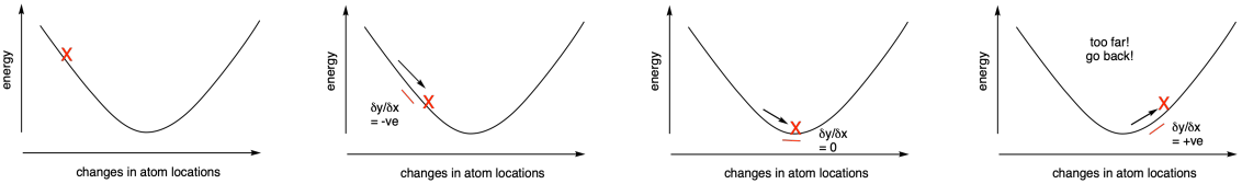
Rather than performing a single calculation, all of these calculations are iterative. For example, the program will determine the energy of the molecule given a set of atom locations (such as the x, y and z coordinates of each atom). It will then make slight changes in atom locations and try again. If the energy goes down, it will keep making changes in the same direction and do the calculations again. If the energy goes up, it has gone too far. It will go back to reach the minimum energy structure.
Figure MK11.1. A series of calculated energies (X) with changing atom positions.
This approach to computational chemistry is based on something called "variational theorem". It basically states that we can take a first guess at the wavefunctions involved in a quantum mechanical calculation and use them to make a rough approximation of the energy. Our first trial will always lead to an energy that is too high, but we can keep improving our approximation over and over until we get closer and closer to the true value of the energy. As we get closer to that minimum energy, and the changes in energy get smaller and smaller each time we change the geometry, the calculation is said to have "converged" on the true value, and we can finish.
Measuring the derivative - the change in slope of the energy vs. atom location curve - can tell us as we approach the energy minimum because the slope will level out at the bottom of the curve. The derivative will approach zero. Some methods use what is called a second derivative approach to looking for this energy minimum. By tracking the change in derivative across the curve, we can more quickly reach the minimum. That's because the slope should start increasing in the region of the bottom of the curve: it will go from a negative slope towards a more positive slope, for example.
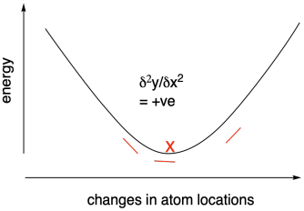
Figure MK11.2. Using a positive second derivative to find an energy minimum.
The idea that we are looking for an energy minimum helps make sure we are on the right track when we want to investigate the structure and energy of a given compound. Sometimes, however, we might end up in a "local minimum". That means energy increases when we change coordinates in either direction, even though an even lower energy structure lies elsewhere. The lower energy structure is called the "global minimum", and the increase in energy between these structures is essentially a barrier for conversion from one less stable structure to another more stable one.
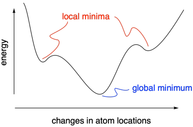
Figure MK11.3. The difference between a local minimum and a global minimum.
Using computational chemistry, we can calculate the structures and relative energies of reactants, products, and intermediates in a reaction. We can even calculate the energy of transition states, although that's a much more difficult task. It's more difficult because we aren't relying on the variational theorem to guide us to the right structure. We are actually going in the opposite direction, looking for an energy maximum. However, we can use a similar approach in monitoring the slope of the curve to find that maximum.
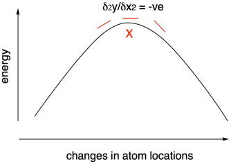
Figure MK11.4. Using a negative second derivative to find a transition state.
If you take a look at a potential energy surface, you will find that a transition state actually lies at a "saddle point" along the energy surface. Although it is a maximum along the coordinate that is changing during a reaction, it is a minimum in the orthogonal direction. Remember, we will always take the lowest-energy path from reactants to products, a little like taking a mountain pass from one valley to another. Instead of traveling over the very top of the mountains, we will still have higher mountains on either side of us as we go over the pass.
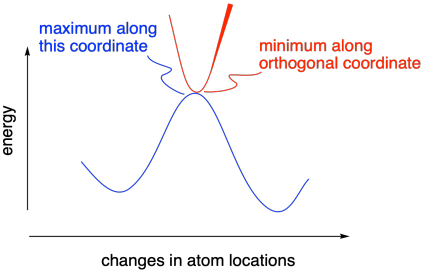
Figure MK11.5. A transition state occurs at a saddle point.
Searching for that saddle point can greatly facilitate finding a transition state. However, we would gain a lot of confidence if we could somehow confirm that we had the right structure and energy. For example, if we had kinetic evidence of the height of the activation barrier in a reaction, we could compare that energy difference to the difference in calculated energies of the reactant and the transition state. This practice of calibrating computational results against experimental energy differences is actually quite common, and results of computational chemistry are often used to extend what we know from experiment.
Problem MK11.1.
a) Based on your knowledge of cyclohexane conformation, indicate where each of the following structures would fall on the potential energy curve provided.

b) Describe each structure as corresponding to a local minimum, a global minimum, or a maximum in energy.
Problem MK11.2.
a) Based on your knowledge of nucleophilic aliphatic substitution, indicate where each of the following structures would fall on the potential energy curve provided.

b) Describe each structure as corresponding to a local minimum, a global minimum, or a maximum in energy.
Problem MK11.3.
a) Based on your knowledge of cationic intermediates, indicate where each of the following structures would fall on the potential energy curve provided.

b) Describe each structure as corresponding to a local minimum, a global minimum, or a maximum in energy.
This site is written and maintained by Chris P. Schaller, Ph.D., College of Saint Benedict / Saint John's University (with contributions from other authors as noted). It is freely available for educational use.

Structure & Reactivity in Organic, Biological and Inorganic Chemistry by Chris Schaller is licensed under a Creative Commons Attribution-NonCommercial 3.0 Unported License.
Send corrections to cschaller@csbsju.edu
Navigation: