CHAPTER 5 - BINDING

C:  MODEL BINDING SYSTEMS

BIOCHEMISTRY - DR. JAKUBOWSKI

3/29/16

C3.  Mathematical Analysis of Cooperative Binding - Hill Plot

Previously we have shown that the binding of oxygen to Mb, which can be described by the equilibrium,

M + L <=> ML, can be described mathematically by

1)  Y = L/[Kd +L].

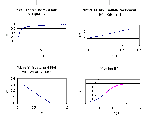
This is the equation of a hyperbola. Remember, that this hyperbolic plot can be transformed in a variety of ways, as summarized in the graphs below for Mb.

Figure:  4 Ways to plot Mb and O2 plots  

How does the sigmoidal binding curve for Hb arise. At least three  models (Hill, MWC, and KNF) can be developed that give rise to sigmoidal binding curves. Remember, sigmoidal curves imply cooperative binding of oxygen to Hb: As oxygen binds, the next oxygen seems to bind with higher affinity (lower Kd)

Hill Model: In this model, we base our mathematical analysis on the fact that the stoichiometry of binding is not one to one, but rather 4 to 1: Perhaps a more useful equation to express the equilibrium would be M + 4L <=> ML4. For this equilibrium, we can derive an equation analogous to the equation 1 above. This equation is:
2)   Y = L4/[Kd + L4].

For any given L and Kd, a corresponding Y can be calculated. Using this equation, the plot of Y vs L is not hyperbolic but sigmoidal (see next link below).  Hence we're getting closer to modeling that actual data.  However, there is one problem.  This sigmoidal curve does not give a great fit to the actual oxygen binding curve for Hb.   Maybe a better fit can be achieved by altering the exponents in equation 2. A more general equation for binding might be M + nL <=> MLn, which gives the following equation:

3)   Y = Ln/[Kd + Ln].

If n is set to 2.8, the theoretical curve of Y vs L gives the best but still not perfect fit to the experimental data.  It must seem arbitrary to change the exponent which seems to reflect the stoichiometry of binding. What molecular interpretation could you give to 2.8Consider another meaning of the equilbrium described above:
M + 4L <=> ML4. One interpretation of this is that all 4 oxygens bind at once to Hb. Or, alternatively, the first one binds with some low affinity, which through associated conformational changes changes the remaining 3 sites to very high affinity sites which immediately bind oxygen if the oxygen concentration is high enough. This model implies what is described as infinitely cooperative binding of oxygen.

(Notice that this equation becomes: Y = L/[Kd + L], when n =1 (as in the case with myoglobin, and in any equilbrium expression of the form:  M  +   L  <==>  ML.  Remember plots of ML vs L or Y vs L gives hyperbolas, with Kd = L at Y = 0.5.)

Does Kd = L at Y = 0.5?    The oxygen concentration at which Y = 0.5 is defined as P50. We can substitute this value into equation 3 which gives an operational definition of Kd in terms of P50.
Y = 0.5 = P50n/[Kd + P50n] - multiple both sides by 2
1 = 2P50n/[Kd + P50n]
Kd + P50n = 2P50n
4)  Kd = P50n
Note that for equation 3,  Kd is not the ligand concentration at half-saturation as we saw in the case with hyperbolic binding curves.

Wolfram Mathematica CDF Player - Hill Model (free plugin required)

  Interactive SageMath Graph: Hill Plot

Now consider another model:

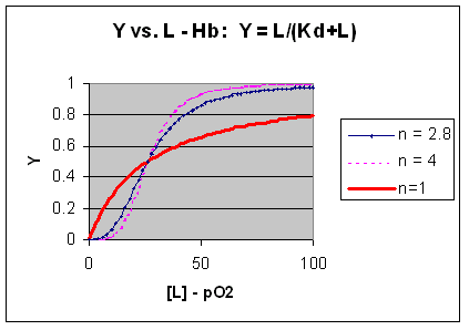
M + L <=> ML + L <=> ML2 + L <=> ML3 + L <=> ML4 where the binding of each oxygen to the unligated or increasing ligated Hb has the same Kd. That is, the affinity of each binding site for oxygen does not increase as more sites are bound to oxygen. In this model, n in equation 3 is 1, and the resulting graph is completely hyperbolic. The fact that the experimental data fits the equilbrium M + 2.8L <=> ML2.8 implies that the binding is cooperative but not infinitely cooperative.  Graphs of Y vs L showing these three cases (n=1, 2.8, and 4) are shown below:

Figure:  Plots of Y vs L for Hb with varying degrees of cooperativity:  n = 1, 2. 8, and 4

The general equation 3),  Y = Ln/[Kd + Ln] can be rearranged as shown below:
 
1 - Y = [Kd + Ln]/[Kd + Ln] - Ln/[Kd + Ln] =
 
5)   1 - Y = Kd/[Kd+ Ln]
 
where 1 - Y is the fraction not bound. Solving for Y/[1-Y] by using equations  3 and 5 gives:
 
6)   Y/[1-Y] = {Ln/[Kd + Ln]}/ Kd/[Kd + Ln] = Ln/Kd.

Taking the log of both sides gives:
 
log (Y/1-Y) = log ( Ln/Kd) =
 
7)   log (Y/1-Y) = nlog L - log Kd
 
A plot of log (Y/1-Y) vs log L is called a Hill plot, where n is the Hill coefficient.   This equation is of the form: 
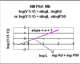
y = mx + b which is a straight line with slope n and y intercept of - log Kd.  When n = 1, as it would be with Mb or Hb when oxygen binds to each site with the same affinity irrespective of the number of other oxygens bound to other sites, the Hill plot is linear with a slope of 1. Solving for the x intercept (when the y axis variable is 0) in equations 7 gives:
 
8)   0 = nlog L -log Kd, or nlogL = log Kd, or log L = (logKd)/n.

The X intercept is when the dependent variable "y" value is 0. This occurs when Y/(1-Y) = 1, which occurs  at half fractional saturation. (Remember log 1 = log 100 = 0)

Substituting equation 4  (Kd = P50n) into (7) and (8) gives
(9) log (Y/1-Y) = nlog L - n log P50 - the Hill Equation with P50 instead of Kd,
(10) 0 = nlog L -nlog P50, or nlogL = nlog P50, or log L = logP50.

Even when n does not equal 1, the Hill plot is linear, since it has the form y=mx+b.  If n = 2.8 or 4, the plot is linear, but has a slope of 2.8 and 4, respectively.    This can be seen in the graph below which shows HIll plots with n = 1, 2.8, and 4.

Figure:  Hill Plot for Mb (n =1)

Hill Plots:  n = 1, 2.8, and 4

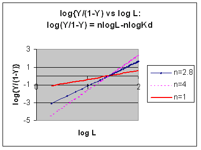
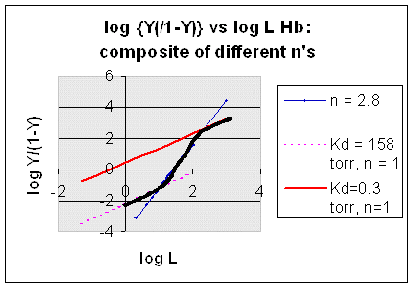
However, the affinity of dixoygen for Hb changes, so that there must be more than one effective Kd.  Hence, the actual Hill  plot of Hb,  log (Y/1-Y) vs log L, can not be linear over all ranges of dioxygen.   A linear plot, such as for Mb, crosses the x axis at one point, with a value of (logKd)/n = logKd since n = 1.  In contrast for Hb, since the Kd seems to change with L concentration, there can not be just 1 value of Kd, as given by the x intercept.  The Hill plot of actual Hb binding data is curvilinear, and cross the x axis only once.  Howver, the ends of the curve (at low and high dioxygen) approach straight lines with slopes of 1 (i.e. n=1).  If extrapolated through the x axis, these lines would give the Kd for the binding of the first and last dioxygens, which bind noncooperatvely.  LogL values near the region of the curve that crosses the x axis approximate a straight line with slope of  2.8.   This implies there is maximal cooperativity in the middle of the binding curve.  The graphs shows that the Kd for the first oxygen binding is much higher than the Kd for the last oxygen binding. Hence the Hill Plots supports our ideas than cooperativity is caused by conformational changes in Hb which occur on oxygen binding such that as progressively more oxygen is bound, the affinity for the remaining sites increases.

Figure:  Hill Plots For Hb Showing straight lines for n=2.8 and for n's=1 which model the low and high affinity sites.

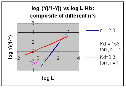
Figurre:  Hill Plot for Hb:  Black line showing hypothetical actual curve

Navigation

Return to Chapter 5C:  Model Binding Sections

Return to Biochemistry Online Table of Contents

 Archived version of full Chapter 5C:  Model Binding Systems