Biochemistry Online: An Approach Based on Chemical Logic

CHAPTER 6 - TRANSPORT AND KINETICS

B: Kinetics of Simple and Enzyme-Catalyzed Reactions

BIOCHEMISTRY - DR. JAKUBOWSKI

4/10/16

Learning Goals/Objectives for Chapter 6B: After class and this reading, students will be able to

write appropriate chemical and differential equations for the rate of disappearance of reactants or appearance of products for 1st order, pseudo first order, second order, reversible first order reactions
draw and interpret graphs for integrated rate equations (showing reactant or product concentrations as a function of time) and initial rate equations (showing the initial velocity vo as a function of reactant ;
derive kinetic rate constants from data and graphs of integrated rate and initial rate equations;
write appropriate chemical, differential equations, and initial rate equations for the rate of disappearance of reactants or appearance of products for simple enzyme catalyzed reaction;
differentiate between rapid and steady state assumptions;
simplify the initial rate equation containing rate constants for an enzyme catalyzed reactions to one replacing the rate constants with kcat and KM, and give operational and mathematical definitions of those constants;

B1. Single Step Reactions

We will first explore the kinetics of non-catalyzed reactions as we did with our study of passive and facilitated diffusion. Before we do that, a brief review of the two major types of kinetic equations that you studied in general chemistry is in order. You learned two methods to analyze kinetic data:

initial velocity method: In this method, the initial rate, v0, is measured as a function of the concentration of reactants. The initial velocity, v0, is the initial slope of a graph of the concentration of reactants or products as a function of time, taken over a range of times such that only a small fraction of A has reacted. Under these condition, [A] over this short range of time is approximately constant and equal to Ao. Initial rate graphs are often based on measurement of product increase with time (dP/dt) so v0 vs A plots have positive slopes. The velocity at time t along the A vs t curve, dA/dt, is constantly changing as [A] decreases since the velocity depend on the [A]. To reiterate, the initial velocity of the reaction is the slope of the initial linear part of the decay curve when the rate is essentiallylinear over a narrow range of A concentrations.
integrated rate method: In this method a differential equation which gives the change of A or P with time (dA/dt or dP/dt) is integrated to give a rate equation giving the concentration of A or P as a function of time. .

REVIEW OF ELEMENTARY REACTION KINETICS

First Order Reaction:

where k1 is the first order rate constant. For these reactions, the velocity of the reaction, v, is directly proportional to [A], or

1a. v = -d[A]/dt = +d[P]/dT = k1[A].

The negative sign in -d[A]/dt indicates that the concentration of A decreases. The equation could also be written as:

1b. v = d[A]/dt = - k1[A].

For the rest of the reactions shown in this chapter, I will follow the convention of writing all velocities expressed as d[x]/dt as positive numbers. A negative sign for a term on the right hand side of the differential equation (as in 1b) will indicate that the concentration dependency of that term will lead to an decrease in [x] with time. Likewise a positive sign for the term on the right hand side of the equation will indicate that concentration dependency of that term will lead to an increase in [x] with time.

Using this nomenclature, the following differential equation can be written and solved to find [A] as a function of t.

dA/dt = -k1A

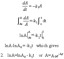
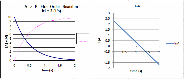
Equation 2 is an example of an integrated rate equation. The following graphs show plots of A vs t and lnA vs t for data from a first order process. Note that the derivative of the graph of A vs t (dA/dt) is the velocity of the reaction. The graph of lnA vs t is linear with a slope of -k1. The velocity of the reaction (slope of the A vs t curve) decreases with decreasing A, which is consistent with equation 1. Again, the initial velocity is determined from data taken in the first part of the decay curve when the rate is linear and little A has reacted. That is [A] is approximately equal to [A0].

Figure: First Order Reaction: A --> P

Once again, for complete clarification, another way of analyzing the kinetics of a reaction, in addition to following the concentration of a reactant or product as a function of time and fitting the data to an integrated rate equation, is to plot the initial velocity, vo, of the reaction as a function of concentration of reactants. The initial velocity is the initial slope of a graph of the concentration of reactants or products as a function of time, taken over a range of times such that only a small fraction of A has reacted, so [A] is approximately constant = Ao. From the first order graph of A vs t above, the slope approaches 0 with increasing time as [A] approaches 0, which clearly indicates that the reaction velocity depends on A. For a first order process, two equivalent equations, 1a and 1b, can be written.

Equation 1a above is written showing the disappearance of A as v = -d[A]/dt = k1[A], while

Equation 1b above is written showing the appearance of A as v = d[A]/dt = -k1[A],

Both equations shows that v is directly proportional to A. As [A] is doubled, the initial velocity is doubled.

Velocity graphs used by biochemists often show the initial velocity of product formation (not reactant decrease) as a function of reactant concentration. Hence, as the concentration of product is increasing, the slopes of initial velocity are positive. A graph of v (= dP/dt) vs [A] for a first order process would have a positive slope and be interpreted as showing that the rate of appearance of P depends linearly on [A].

Second Order/Pseudo First Order Reactions

where k2 is the second order rate constant. For the first of these irreversible reactions, the velocity of the reaction, v, is directly proportional to [A] and [B], or

3. v = d[A]/dt = d[B]/dt = -k2[A][B].

We will consider two special cases of this reaction type:

[B] >> [A]. Under these conditions, [B] never changes, so equation (3) becomes

4. v = -(k2[B]) [A] = -k1' [A]

where k1' is the pseudo first order rate constant (= k2[B] ) for the reaction. The reaction appears to be first order, depending only on [A].

The only reactant is A which must collide with another A to form P, as illustrated in the second reaction above. The derivations below apply to this special case.

The following differential equation can be written and solved to find [A] as a function of t.

5. v = d[A]/dt = +2d[P]/dT = -k2[A][A] = - k2[A]2

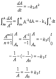
6. 1/A = 1/Ao + k2t

The following graphs show plots of A vs t and 1/A vs t for data from a second order process.

Figure: Second Order Reaction: A + A --> P

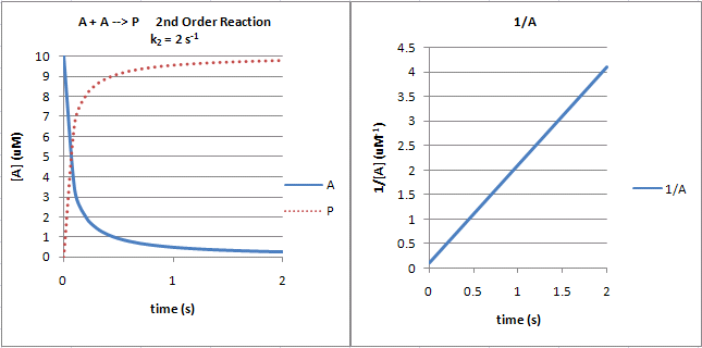
Note that just from a plot of A vs t, it would be difficult to distinguish a first from second order reaction. If the plots were superimposed, you would observe that at the same concentration of A (10 for example as in the linked plots), the vo of a first order reaction would be proportional to 10 but for a second order reaction to 102 or 100. Therefore, the second order reaction is faster (assuming similarity in the relative magnitude of the rate constants) as indicated by the steeper negative slope of the curve. However, at low A (0.1 example), the vo of a first order reaction would be proportional to 0.1 but for a second order reaction to 0.12 or 0.01. Therefore, at low A, the second order reaction is slower.

The interactive graphs below show the first and second order conversion of reactant A to product. Change the slides to see how the curves are different.

4/26/13Wolfram Mathematica CDF Player - Comparison of 1st and 2nd Order Conversion of A --> P (First order - solid line; Second order - dashed line) (free plugin required)

SageMathLogo Interactive SageMath Graph: 1^st and 2^nd order reactions

Navigation

Return to B: Kinetics of Simple and Enzyme-Catalyzed Reactions Sections

Return to Biochemistry Online Table of Contents

Archived version of full Chapter 5B: Kinetics of Simple and Enzyme-Catalyzed Reactions

Biochemistry Online by Henry Jakubowski is licensed under a Creative Commons Attribution-NonCommercial 4.0 International License.