CHAPTER 6 - TRANSPORT AND KINETICS 

 
B:  Kinetics of Simple and Enzyme-Catalyzed Reactions

BIOCHEMISTRY - DR. JAKUBOWSKI

4/10/16

B8.  Experimental Determination of Vmax and Km  

How can  Vm and  Km  be determined from experimental data? 

a.  From initial rate data:  The most common way is to determine initial rates, v0, from experimental values of P or S as a function of time.  Hyperbolic graphs of v0 vs [S] can be fit be fit or transformed as we explored with the different mathematical transformations of the hyperbolic binding equation to determine Kd.  These included:

• nonlinear hyperbolic fit

• double reciprocal plot

• Scatchard plot

The double-reciprocal plot is commonly used to analyze initial velocity vs substrate concentration data.  When used for such purposes, the graphs are referred to as Lineweaver-Burk plots, where plots of 1/v vs 1/S are straight lines with slope m = Km/Vmax, and y intercept b = 1/Vmax. 

Interactive SageMath Graph: Lineweaver Burk Plot

These plots can not be analyzed using linear regression, however, since that method assumes constant error in the y axis (in this case 1/v) data.  A weighted linear regression or even better, a nonlinear fit to a hyperbolic equation should be used.  The Mathcad template below shows such a nonlinear fit.  A rearrangement of the corresponding Scatchard equations in the Eadie-Hofstee plot is also commonly used, especially to visualize enzyme inhibition data as we will see in the next chapter.

Mathcad 8 - Nonlinear Hyperbolic Fit.  Vm and Km.

Common Error in Biochemistry Textbooks:  The Shape of the Hyperbola

b.  From integrated rate equations:  KM and Vm can be extracted from progress curves of A or P as a function of t at one single A0 concentration by deriving an integrated rate equation for A or P as a function of t, as we did in equation 2 which shows the integrated rate equation for the conversion of A --> P in the absence of enzyme.  In principle this method would be better than the initial rates methods.  Why?  One reason is that is not easy to be certain you are measuring the initial rate for each and every [S] which should vary over a wide range.  It's also time intensive. In addition, think how much of the data is discarded if you take an entire progress curve at each substrate concentration, especially if you quench the reaction at a given time point, which effectively limits the data to one time point per substrate. 

In practice, the mathematics are complicated as it is not possible to get a simple explicit function of [P] or [S] as a function of time.   Nevertheless, progress has been made in progress curve analysis (no pun intended).  Let us consider the simple case of a single substrate S (or A) being converted to product P in an enzyme catalyzed reaction.  The analogous equations for first order, non-catalyzed rates were
A=Aoe-k1t or P = A0(1-e-k1t). 

Now let's derive the equations for the enzyme-catalyzed reaction. 

The derivation of the relevant equations are shown below. 

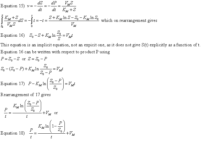
A graph of P/t vs [ln (1-P/S0)]/t (shown below) from equation 18 gives a straight line with a slope of Km and a y intercept of Vm.   Note that the calculated values of Vm and Km are derived from only one substrate concentration, and the values may be affected by product inhibition

Figure:  Enzyme Kinetics Progress Curve

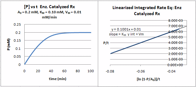
A comparison of the progress curves for the noncatalyzed 1st order reaction of S to P (red) and  the enzyme catalyzed reaction (blue) is shown below.  (Many thanks to Gregory Bard, UW Stout, for help with the Sage Math code).   Note that the curves are similar but different.  Adjust the sliders to better compare the two.  If you didn't know an enzyme was present, you could easily fit the data to a first order rise in [P] with time, but it would not be the optimal fit.  The progress curve in the presence of enzyme is ideal in that product inhibition is not part of the model, which would greatly complicate the analysis.

Interactive SageMath Graph: [P] vs t for enzyme catalyzed (blue) and non-enzyme catalyzed 1st order conversion, S to P

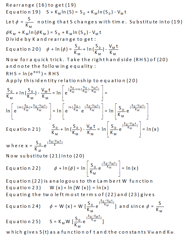
Can a simple explicit equation of P vs t be derived?  The answer is no.  However it can be represented by an explicit Lambert function as shown in the derivation below.

Navigation

Return to B:  Kinetics of Simple and Enzyme-Catalyzed Reactions Sections

Return to Biochemistry Online Table of Contents

Archived version of full Chapter 5B:  Kinetics of Simple and Enzyme-Catalyzed Reactions