CHAPTER 6 - TRANSPORT AND KINETICS

C: ENZYME INHIBITION

BIOCHEMISTRY - DR. JAKUBOWSKI

06/12/2014

C2. Competitive Inhibition

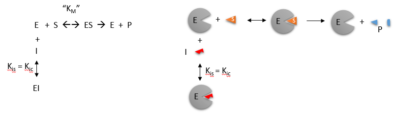
Reversible Competitive inhibition occurs when substrate (S) and inhibitor (I) both bind to the same site on the enzyme. In effect, they compete for the active site and bind in a mutually exclusive fashion. This is illustrated in the chemical equations and molecular cartoon below.

There is another type of inhibition that would give the same kinetic data.  If S and I bound to different sites, and S bound to E and produced a conformational change in E such that I could not bind (and vice versa), then the binding of S and I would be mutually exclusive. This is called allosteric competitive inhibition. Inhibition studies are usually done at several fixed and non-saturating concentrations of I and varying S concentrations.

The key kinetic parameters to understand are Vm and Km. Let us assume for ease of equation derivation that I binds reversibly, and with rapid equilibrium to E, with a dissociation constant Kis. The "s" in the subscript "is" indicates that the slope of the 1/v vs 1/S  Lineweaver-Burk plot changes while the y intercept stays constant.  Kis is also named K_ic where the subscript "c" stands for competitive inhibition constant.

A look at the top mechanism shows that even in the presence of I, as S increases to infinity, all E is converted to ES. That is, there is no free E to which I could bind. Now remember that Vm= kcatEo. Under these condition, ES = Eo; hence v = Vm.   Vm is not changed. However, the apparent Km, Kmapp, will change. We can use LaChatelier's principle to understand this. If I binds to E alone, and not ES, it will shift the equilibrium of E + S <==> ES to the left, which would have the affect of increasing the Km app (i.e. it would appear that the affinity of E and S has decreased.). The double reciprocal plot (Lineweaver Burk plot) offers a great way to visualize the inhibition. In the presence of I, Vm does not change, but Km appears to increase. Therefore, 1/Km, the x-intercept on the plot will get smaller, and closer to 0. Therefore the plots will consists of a series of lines, with the same y intercept (1/Vm), and the x intecepts (-1/Km) closer and closer to the 0 as I increases. These intersecting plots are the hallmark of competitive inhibition. 

Note that in the first three inhibition models discussed in this section, the Lineweaver-Burk plots are linear in the presence and absence of inhibitor.  This suggests that plots of v vs S in each case would be hyperbolic and conform to the usual form of the Michaelis Menton equation, each with potentially different apparent Vm and Km values.

An equation, shown in the figure above, can be derived which shows the effect of the competitive inhibitor on the velocity of the reaction. The only change is that the Km term is multiplied by the factor 1+I/Kis. Hence Kmapp = Km(1+I/Kis). This shows that the apparent Km does increase as we predicted. Kis is the inhibitor dissociation constant in which the inhibitor affects the slope of the double reciprocal plot. 

Wolfram Mathematica CDF Player - Competitive Inhibition v vs S (free plugin required)

Interactive SageMath Graph: Competitive Inhibition 1/v  vs 1/S

4/6/14Wolfram Mathematica CDF Player - Competitive Inhibition - Lineweaver Burk(free plugin required)

Interactive SageMath Graph: Competitive Inhibition - Lineweaver Burk

If the data was plotted as vo vs log S, the plots would be sigmoidal, as we saw for plots of ML vs log L in Chapter 5B.   In the case of competitive inhibitor, the plot of  vo vs log S in the presence of different fixed concentrations of inhibitor would consist of a series of sigmoidal curves, each with the same Vm, but with different apparent Km values (where Kmapp = Km(1+I/Kis), progressively shifted to the right.   Enyzme kinetic data is rarely plotted this way, but simple binding data for the M + L < == > ML equilibrium, in the presence of different inhibitor concentrations is. 

Reconsider our discussion of the simple binding equilibrium, M + L <==> ML.  When we wished to know how much is bound, or the fractional saturation, as a function of the log L, we considered  three examples.

1. L = 0.01 Kd (i.e. L << Kd), which implies that Kd = 100L.  Then Y = L/[Kd+L] = L/[100L + L] ≈1/100.  This implies that irrespective of the actual [L], if L = 0.01 Kd, then Y ≈0.01. 
2. L = 100 Kd (i.e. L >> Kd), which implies that Kd = L/100.  Then Y = L/[Kd+L] = L/[(L/100) + L] = 100L/101L ≈ 1.  This implies that irrespective of the actual [L], if L = 100 Kd, then Y ≈1.
3. L = Kd, then Y = 0.5

These scenarios show that if L varies over 4 orders of magnitude (0.01Kd < Kd < 100Kd), or, in log terms, from
-2 + log Kd < log Kd  < 2 + log Kd),  irrespective of the magnitude of the Kd, that Y varies from approximately 0 - 1. 

In other words, Y varies from 0-1 when L varies from log Kd by +2.  Hence, plots of Y vs log L for a series of binding reactions of increasingly higher Kd (lower affinity) would reveal a series of identical sigmoidal curves shifted progressively to the right, as shown below. 

The same would be true of vo vs S in the presence of different concentration of a competitive inhibitor, for initial flux, Jo vs ligand outside, in the presence of a competitive inhibitor, or ML vs L (or Y vs L) in the presence of a competitive inhibitor.

Wolfram Mathematica CDF Player - Competitive Inhibition v vs logS (free plugin required)

In many ways plots of v0 vs lnS are easier to visually interpret than plots of v0 vs S .  As noted for simple binding plots, textbook illustrations of hyperbolas are often misdrawn, showing curves that level off too quickly as a function of [S] as compared to plots of  v0 vs lnS, in which it is easy to see if saturation has been achieved.  In addition, as the curves above show, multiple complete plots of v0 vs lnS at varying fixed inhibitor concentration or for variant enzyme forms (different isoforms, site-specific mutants) over a broad range of lnS can be made which facilitates comparisons of the experimental kinetics under these different conditions.  This is especially true if Km values differ widely. 

Now that you are more familiar with binding, flux, and enzyme kinetics curves, in the presence and absence of inhibitors, you should be able to apply the above analysis to inhibition curves where the binding, initial flux, or the initial velocity is plotted at varying competitive inhibitor concentration at different  fixed concentration nonsaturating concentrations of ligand or substrate. Consider the activity of an enzyme.  Lets say that at some reasonable concentration of substrate (not infinite), the enzyme is approximately 100% active. If a competitive inhibitor is added, the activity of the enzyme would drop until at saturating (infinite) I, no activity would remain.  Graphs showing this are shown below.

Figure:  Inhibition of Enzyme Activity - % Activity vs log [Inhibitor]

A special case of competitive inhibition: the specificity constant:  In the previous chapter, the specificity constant was defined as kcat/KM which we also described as the second order rate constant associated with the bimolecular reaction of E and S when S << KM.  It also describes how good an enzyme is in differentiating between different substrates.  If has enzyme encounters two substrates, one can be considered to be a competitive inhibitor of the other.  The following derivation shows that the ratio of initial velocities for two competing substrates at the same concentration is equal to the ratio of their kcat/KM values.

Java Applet: Competitive Inhibition I;   Competitive Inhibition II

Navigation

Return to Chapter 6C:  Enzyme Inhibition Sections

Return to Biochemistry Online Table of Contents

Archived version of full Chapter 6C:  Enzyme Inhibition