Biochemistry Online: An Approach Based on Chemical Logic
CHAPTER 2 - PROTEIN STRUCTURE
G: PREDICTING PROTEIN PROPERTIES FROM SEQUENCES
BIOCHEMISTRY - DR. JAKUBOWSKI
Last Update: 3/9/16
|
Learning Goals/Objectives for Chapter 2G: After class and this reading, students will be able to:
|
G1. Introduction to Bioinformatics, Computational Biology and Proteomics
With the solving of the human genome, intensive effort has been devoted to analysis of the human genome to determine the number and transcriptional regulation of the encoded genes. Much has been learned from comparative genomics, as genomes from mice, rats, chimpanzees, and a variety of prokaryotes are compared in an effort to help understand the nature of genes and their transcriptional regulation. The vast amount of genomic data that has to be "mined" has required the development of computational and computer programs to enable the analysis. Two relatively new fields have subsequently arisen: bioinformatics and computational biology. (In a personal note, the words computational biology seem somewhat restrictive since the field of computational chemistry, which has a longer history, has significant overlap with "computational biology". I prefer computational biochemistry). These fields have significant overlap (as do physical chemistry/chemical physics and biochemistry/molecular biology/chemical biology), so I defer to others to define them.
The NIH Biomedical Information Science and Technology Initiative Consortium: "This consortium has agreed on the following definitions of bioinformatics and computational biology, recognizing that no definition could completely eliminate overlap with other activities or preclude variations in interpretation by different individuals and organizations.
Bioinformatics: Research, development, or application of computational tools and approaches for expanding the use of biological, medical, behavioral or health data, including those to acquire, store, organize, archive, analyze, or visualize such data.
Computational Biology: The development and application of data-analytical and theoretical methods, mathematical modeling and computational simulation techniques to the study of biological, behavioral, and social systems."
This web book has been developed as a first semester biochemistry text and choices have been made to limit the scope of the material to exclude content covered in detail in a molecular biology/genetics class. Hence, this text will not discuss in significant detail the genome and transcriptome, and mechanisms of replication, transcription, or translation. However, with its emphasis on protein structure and function, proteomics, the characterization of structure and function of all proteins within a cell, is a logical candidate for inclusion.
In the last several years, computational biology/chemistry and web-based programs have become available for the systematic analysis of individual proteins, and for the comparative analysis of many proteins, based on either their DNA or amino acid sequence. Clearly the ultimate goal in the description of a protein would be to determine, from the amino acid or nucleotide sequence, the three dimensional structure of a protein and its biological function, including all its binding partners.
Here is a list of proteome web resources and tutorials
- Bioinformatics and Homology Modeling: A Student-Tested Tutorial for Beginners
- ExPASy Proteomics Portal
- Animations: Proteins and Proteomics
- Protein Matchmaking - Protein Data Base Search Engine: allows superposition of similar protein structures
- SIB: Swiss Institute of Bioinformatics:
- Protein Structure and Proteome Analysis
Voluminous databases of biomolecule sequence and structural data, as well as analysis software packages, are available at a variety of web sites, including:
- BioGrid: General Repository for Interaction (protein, NA) Datasets
- GenBank: DNA sequence database (over 100 billion bases as of 9/05), from the NCBI
- BLAST finds regions of similarity between biological sequences
- UniProtKB/Swiss-Prot: manually annotated and reviewed section of the UniProt Knowledgebase (UniProtKB)
- ProSite: database of protein families and domains. It consists of biologically significant sites, patterns and profiles that help to reliably identify to which known protein family (if any) a new sequence belongs. From the Swiss Institute of Bioinformatics
- Swiss-2D Gel Database: from the Swiss Institute of Bioinformatics
- RSCB Protein Data Bank: Protein and nucleic acid 3D structures from x-ray crystallography and NMR spectroscopy (about 33,000 as of 9/15/05)
- SWISS-MODEL Repository: 3D comparative protein structure models (675,000) generated by the fully automated homology-modeling pipeline SWISS-MODEL. (again from Swiss Institute of Bioinformatics)
- ExPASy (Expert Protein Analysis System) server of the Swiss Institute of Bioinformatics
The NCBI has an extensive array of available tools (free), including:
- literature databases: including word searches in many books
- All resources: including nucleotide, protein, structure, genome, chemical
- Entrez: the life science search engine
- Blast Quick Start: easy way to start a BLAST search
- complete human proteome from UniProtKB/Swiss-Prot
A summary of three important sites:
• NCBI-Protein:
The Protein database is a collection of sequences from several sources,
including translations from annotated coding regions in GenBank, RefSeq
and TPA, as well as records from SwissProt, PIR, PRF, and PDB. Protein
sequences are the fundamental determinants of biological structure and
function
• Uniprot: The
UniProt Knowledgebase (UniProtKB) is the central hub for the collection
of functional information on proteins, with accurate, consistent and
rich annotation. In addition to capturing the core data mandatory for
each UniProtKB entry (mainly, the amino acid sequence, protein name or
description, taxonomic data and citation information), as much
annotation information as possible is added.
•
Gene Card: GeneCards is a
searchable, integrative database that provides comprehensive,
user-friendly information on all annotated and predicted human genes. It
automatically integrates gene-centric data from ~125 web sources,
including genomic, transcriptomic, proteomic, genetic, clinical and
functional information
The table below (directly taken from Wikipedia) shows some of the incredible information available the proteome and genome of each human chromosome.
Table: Human proteome and genome from
Wikipedia
(Data source:
Ensembl genome browser release 68, July 2012)
| Chromsome | Length (mm) | BP | Variations | Confirmed Proteins | Putative Proteins | Pseudogenes | miRNA | rRNA | snRNA | snoRNA | misc ncRNA | Links |
| 1 | 85 | 249,250,621 | 4,401,091 | 2,012 | 31 | 1,130 | 134 | 66 | 221 | 145 | 106 | EBI |
| 2 | 83 | 243,199,373 | 4,607,702 | 1,203 | 50 | 948 | 115 | 40 | 161 | 117 | 93 | EBI |
| 3 | 67 | 198,022,430 | 3,894,345 | 1,040 | 25 | 719 | 99 | 29 | 138 | 87 | 77 | EBI |
| 4 | 65 | 191,154,276 | 3,673,892 | 718 | 39 | 698 | 92 | 24 | 120 | 56 | 71 | EBI |
| 5 | 62 | 180,915,260 | 3,436,667 | 849 | 24 | 676 | 83 | 25 | 106 | 61 | 68 | EBI |
| 6 | 58 | 171,115,067 | 3,360,890 | 1,002 | 39 | 731 | 81 | 26 | 111 | 73 | 67 | EBI |
| 7 | 54 | 159,138,663 | 3,045,992 | 866 | 34 | 803 | 90 | 24 | 90 | 76 | 70 | EBI |
| 8 | 50 | 146,364,022 | 2,890,692 | 659 | 39 | 568 | 80 | 28 | 86 | 52 | 42 | EBI |
| 9 | 48 | 141,213,431 | 2,581,827 | 785 | 15 | 714 | 69 | 19 | 66 | 51 | 55 | EBI |
| 10 | 46 | 135,534,747 | 2,609,802 | 745 | 18 | 500 | 64 | 32 | 87 | 56 | 56 | EBI |
| 11 | 46 | 135,006,516 | 2,607,254 | 1,258 | 48 | 775 | 63 | 24 | 74 | 76 | 53 | EBI |
| 12 | 45 | 133,851,895 | 2,482,194 | 1,003 | 47 | 582 | 72 | 27 | 106 | 62 | 69 | EBI |
| 13 | 39 | 115,169,878 | 1,814,242 | 318 | 8 | 323 | 42 | 16 | 45 | 34 | 36 | EBI |
| 14 | 36 | 107,349,540 | 1,712,799 | 601 | 50 | 472 | 92 | 10 | 65 | 97 | 46 | EBI |
| 15 | 35 | 102,531,392 | 1,577,346 | 562 | 43 | 473 | 78 | 13 | 63 | 136 | 39 | EBI |
| 16 | 31 | 90,354,753 | 1,747,136 | 805 | 65 | 429 | 52 | 32 | 53 | 58 | 34 | EBI |
| 17 | 28 | 81,195,210 | 1,491,841 | 1,158 | 44 | 300 | 61 | 15 | 80 | 71 | 46 | EBI |
| 18 | 27 | 78,077,248 | 1,448,602 | 268 | 20 | 59 | 32 | 13 | 51 | 36 | 25 | EBI |
| 19 | 20 | 59,128,983 | 1,171,356 | 1,399 | 26 | 181 | 110 | 13 | 29 | 31 | 15 | EBI |
| 20 | 21 | 63,025,520 | 1,206,753 | 533 | 13 | 213 | 57 | 15 | 46 | 37 | 34 | EBI |
| 21 | 16 | 48,129,895 | 787,784 | 225 | 8 | 150 | 16 | 5 | 21 | 19 | 8 | EBI |
| 22 | 17 | 51,304,566 | 745,778 | 431 | 21 | 308 | 31 | 5 | 23 | 23 | 23 | EBI |
| X | 53 | 155,270,560 | 2,174,952 | 815 | 23 | 780 | 128 | 22 | 85 | 64 | 52 | EBI |
| Y | 20 | 59,373,566 | 286,812 | 45 | 8 | 327 | 15 | 7 | 17 | 3 | 2 | EBI |
| mtDNA | 0.0054 | 16,569 | 929 | 13 | 0 | 0 | 0 | 2 | 0 | 0 | 22 | EBI |
This chapter will describe programs that allow predictions of secondary and tertiary structures of proteins. Specific exercises using web-based bioinformatics programs can be found at the end.
G2. Prediction of Secondary Structure
As we have seen previously, amino acids vary in their propensity to be found in alpha helices, beta strands, or reverse turns (beta bends, beta turns). These difference can be rationalized from the structure of each amino acid, as described before.
Figure: Amino Acid Structure and propensity for secondary structure
From the data bases, propensities can be calculated to determine the likelihood that a given amino acid will be in one of those structures. Glycine for example would have a high propensity to be in reverse turns, while Pro, a helix breaker, would have a low propensity to be in an alpha helix. A number is assigned to each amino acid for each category of secondary structure. High numbers favor the likelihood that that amino acid would be in that structure. One of the earliest propensity scales was from Chou-Fasman, where H indicates high propensity for secondary structure, h intermediate propensity, i is inhibitory, b is a intermediate breaker, and B is a significant breaker of secondary structure.
Chou-Fasman Amino Acid Propensities
| A.A. | Helix | Sheet | ||
| Designation | P | Designation | P | |
| Ala | H | 1.42 | i | 0.83 |
| Cys | i | 0.70 | h | 1.19 |
| Asp | I | 1.01 | B | 0.54 |
| Glu | H | 1.51 | B | 0.37 |
| Phe | h | 1.13 | h | 1.38 |
| Gly | B | 0.57 | b | 0.75 |
| His | I | 1.00 | h | 0.87 |
| Ile | h | 1.08 | H | 1.60 |
| Lys | h | 1.16 | b | 0.74 |
| Leu | H | 1.21 | h | 1.30 |
| Met | H | 1.45 | h | 1.05 |
| Asn | b | 0.67 | b | 0.89 |
| Pro | B | 0.57 | B | 0.55 |
| Gln | h | 1.11 | h | 1.10 |
| Arg | i | 0.98 | i | 0.93 |
| Ser | i | 0.77 | b | 0.75 |
| Thr | i | 0.83 | h | 1.19 |
| Val | h | 1.06 | H | 1.70 |
| Trp | h | 1.08 | h | 1.37 |
| Tyr | b | 0.69 | H | 1.47 |
Next a stretch or "window" of amino acids about 7 amino acids is taken, starting from the N-terminal of the protein. First the average alpha helical propensities for amino acids 1-7 are determined and assigned, let's say, to the middle (4th) amino acid in that sequence. Then alpha helical propensities for amino acids 2-8 (the next window) are averaged and assigned to the middle (5) amino acid in that range. The window slide down the protein sequence until all but the first and last few amino acids have an average value assigned to them. If a contiguous stretch of amino acids has high average propensity, they are probably in an alpha helix in the native protein. This process is repeated using beta strand and reverse turn propensities. The final assignments of most probably secondary structure are made. Of course this system was tested against proteins whose tertiary structure was known. See the results for secondary structure prediction for one protein. In this example, the average propensity for four contiguous amino acids is calculated (starting with amino acids 1-4, then amino acids 5-8, etc, and continuing to the end of the polypeptide). Next this process is repeated for contiguous stretches 2-5, 6-9, etc, and continuing to the end. The original Chou Fasman propensities have been updated using known protein structure to give better predictions.
- Chou Fasman Online Secondary Structure Predictor
Additional information about putative helices can be obtained by determining if they are amphiphilic (one side of the helix containing mostly hydrophobic side chains, with the opposite side containing polar or charged side chains. A helical wheel projection can be made. In this a circle is draw representing a downward cross-sectional view of the helix axis.
Figure: Helical wheel projection
The side chains are placed on the outside of the circle, staggered in a fashion determined by the fact that there are 3.6 amino acids per turn of the helix. If one side of the wheel contains predominantly nonpolar side chains while the other side has polar side chains, the helix is amphiphilic. Imagine how such helices might be packed in a protein.
- Helical wheel predictor | Another Helical wheel predictor | Another
- Programs for Secondary Structure Prediction
G3. Prediction of Hydrophobicity
In a completely analogous fashion, a hydrophobic propensity or hydopathy can be calculated. In this system, empirical measures of the hydrophobic nature of the side chains are used to assign a number to a given amino acid. Many hydropathy scales are used. Several are based on the Dmo transfer of the side chains from water to a nonpolar solvent. Two commonly used scales are the Kyte-Doolittle Hydropathy and Hopp-Woods scales (used more like a hydrophilicity index to predict surface or water accessible structures that might be recognized by the immune system)
Hydrophobicity Indices for Amino Acids
|
Amino Acid |
Kyte-Doolittle |
Hopp-Woods |
|
Alanine |
1.8 |
-0.5 |
|
Arginine |
-4.5 |
3.0 |
|
Asparagine |
-3.5 |
0.2 |
|
Aspartic acid |
-3.5 |
3.0 |
|
Cysteine |
2.5 |
-1.0 |
|
Glutamine |
-3.5 |
0.2 |
|
Glutamic acid |
-3.5 |
3.0 |
|
Glycine |
-0.4 |
0.0 |
|
Histidine |
-3.2 |
-0.5 |
|
Isoleucine |
4.5 |
-1.8 |
|
Leucine |
3.8 |
-1.8 |
|
Lysine |
-3.9 |
3.0 |
|
Methionine |
1.9 |
-1.3 |
|
Phenylalanine |
2.8 |
-2.5 |
|
Proline |
-1.6 |
0.0 |
|
Serine |
-0.8 |
0.3 |
|
Threonine |
-0.7 |
-0.4 |
|
Tryptophan |
-0.9 |
-3.4 |
|
Tyrosine |
-1.3 |
-2.3 |
|
Valine |
4.2 |
-1.5 |
For a water-soluble protein, a continuous stretch of amino acids found to have a high average hydropathy is probably buried in the interior of the protein. Consider the example of bovine a-chymotrypsinogen, a 245 amino acid protein, whose sequence is shown below in single letter code.
1
CGVPAIQPVLSGLSRIVNGEEAVPGSWPWQVSLQDKTGFHFCGGSLINENWVVTAAHCGV
61
TTSDVVVAGEFDQGSSSEKIQKLKIAKVFKNSKYNSLTINNDITLLKLSTAASFSQTVSA
121
VCLPSASDDFAAGTTCVTTGWGLTRYTNANTPDRLQQASLPLLSNTNCKKYWGTKIKDAM
181
ICAGASGVSSCMGDSGGPLVCKKNGAWTLVGIVSWGSSTCSTSTPGVYARVTALVNWVQQ
241 TLAAN
A hydrophathy plot for chymotrypsinogen (sum of hydropathies of seven consecutive residues) shows many stretches that are presumably buried in the interior of the protein.
Figure: hydrophathy plot for chymotrypsinogen
G4. Prediction of Membrane Protein Structure
So far we have discussed predominantly globular proteins that are soluble in water. Proteins are also found associated with membranes. Two major classes of membrane proteins are found in nature.
- peripheral membrane proteins: water soluble proteins bound reversibly and non-covalently to the membrane through electrostatic attractions between charged polar head groups of the phospholipids and the protein. These proteins can often be released from the membrane by addition of high salt, since they are often attracted to the bilayer by electrostatic interactions between charged phospholipid head groups and polar/charged groups on the protein surface.
- integral membrane proteins: actually insert into the bilayer. These can be released from the membrane and effectively solubilized by the addition of single chain amphiphiles (detergents) which form a mixed micelle with the integral membrane protein. Nonionic detergents (Trition X-100, octylglucoside, etc) are often used in the purification of membrane proteins. Ionic detergents (like SDS) not only solubilize the integral membrane proteins, but also denature them.
Figure: Types of membrane proteins
In some of these integral membrane proteins, large extracellullar and intracellular domains of the protein are present, connected by the intramembrane regions. The intramembrane spanning region often consists of either a single alpha helix, or 7 different helical regions which zig-zag through the membrane. These transmembrane sequences can readily be determined through hydropathy calculations. For example, consider the integral membrane bovine protein rhodopsin. Its 348 amino acid sequence (in single letter code) is shown below:
MNGTEGPNFYVPFSNKTGVVRSPFEAPQYYLAEPWQFSMLAAYMFLLIMLGFPINFLTLY
VTVQHKKLRTPLNYILLNLAVADLFMVFGGFTTTLYTSLHGYFVFGPTGCNLEGFFATLG
GEIALWSLVVLAIERYVVVCKPMSNFRFGENHAIMGVAFTWVMALACAAPPLVGWSRYIP
EGMQCSCGIDYYTPHEETNNESFVIYMFVVHFIIPLIVIFFCYGQLVFTVKEAAAQQQES
ATTQKAEKEVTRMVIIMVIAFLICWLPYAGVAFYIFTHQGSDFGPIFMTIPAFFAKTSAV
YNPVIYIMMNKQFRNCMVTTLCCGKNPLGDDEASTTVSKTETSQVAPA
Rhodopsin hydropathy plot calculations shows that is contains seven transmembrane helices which wind through the membrane in a serpentine fashion..
Figure: Rhodopsin hydropathy plot
Figure: seven transmembrane helices
Rhodopsin Hydropathy Results
| No. | N terminal | transmembrane region | C terminal | type | length |
| 1 | 40 | LAAYMFLLIMLGFPINFLTLYVT | 62 | PRIMARY | 23 |
| 2 | 71 | PLNYILLNLAVADLFMVFGGFTT | 93 | SECONDARY | 23 |
| 3 | 113 | EGFFATLGGEIALWSLVVLAIER | 135 | SECONDARY | 23 |
| 4 | 156 | GVAFTWVMALACAAPPLVGWSRY | 178 | SECONDARY | 23 |
| 5 | 207 | MFVVHFIIPLIVIFFCYGQLVFT | 229 | PRIMARY | 23 |
| 6 | 261 | FLICWLPYAGVAFYIFTHQGSDF | 283 | PRIMARY | 23 |
| 7 | 300 | VYNPVIYIMMNKQFRNCMVTTLC | 322 | SECONDARY | 23 |
In summary, hydropathy plots are hence useful in finding buried regions in water soluble proteins, transmembrane helices in integral membrane proteins as well as short stretches of polar/charged amino acids that might form surface loops recognizable by immune system antibodies. The window size used in hydropathy plots would obviously affect the calculated results. Windows of 20 amino acids are useful to determine transmembrane helices while windows of 5-7 amino acids are used to find surface-exposed hydrophilic sites.
Membrane proteins call be solubilized by addition of single chain amphiphiles (detergents). The nonpolar tails of the detergents interact with the hydrophobic transmembrane domain of the membrane protein forming a "mixed" micelle-like structure. Nonionic detergents like Triton X-100 and octyl-glucoside are often used to solubilize membrane proteins in their near native state. In contrast, ionic detergents like sodium dedecyl sulfate (with a negatively charged head group) denature proteins during the solubilization process. To study membrane proteins in a more native-like environment, proteins solubilized by nonionic detergent can be reconstituted into bilayer liposome structures using methods similar to those from Lab 1 in which you prepared dye-capsulated large unilamellar vesicles (LUVs). However, it can be difficult to study the intra- and extracellular domains of membrane proteins in liposomes, given that one of those domains is hidden inside the liposome. A novel technique that removes this barrier was recently developed by Sligar. He created an amphiphilic protein disc with an opening in the center. The inner opening is lined with nonpolar residues, while the outer surface of the disc is polar. When the discs were added to phosphlipids, small bilayers formed inside the disc. Membrane proteins like the b-2 adrenergic receptor could be reconstituted in the nanodisc bilayers, allowing solvent exposure of both the intracellular and extracellular domains of the receptor protein.
Figure: Nanodisc with membrane protein
- Experimentally Determined Hydropathy Scales
- Protein Sequence Structural Features
- Membrane Protein Resources
- Membrane Proteins of Known 3D Structure
- 57 Different Amino Acid Scale Predictors from ExPASy
G5. Prediction of Protein Tertiary Structure
We are getting closer to predicting the tertiary structure of a protein, but as we have seen from molecular mechanics and dynamics calculations, it is a huge computational task. There are two basic approaches which are often combined.
- calculations using energy minimization and statistical mechanics: These "semi-empirical" techniques don't assume any given secondary structure propensities or hydrophobicities. Such methods have produced limited success with small proteins whose actual structure is known.
- homology modeling based on proteins of known structure: The structures of about 117,00 (3/16) different biological macromolecules are known. This can serve as an empirical data base of possible conformations. Instead of an infinite number of prototypical structures, it is becoming clear that there may be a reasonably low number (in the hundreds) of basic structural motifs that are used over and over in nature. By aligning the amino acid sequences of different proteins, and comparing their properties (such as secondary structure propensities, hydrophobicities, etc.), probable low energy structures of the new protein can be determined. This initial structure can be run through multiple minimization and dynamic simulations to produce a tentative "lowest" energy structure. The structure should be compact (checked through calculation of packing density) and experimental techniques (such as spectroscopic methods) should be employed to validate the structure.
Many mechanisms of the actual folding process have been postulated, most of which have some experimental support. In one, a hydrophobic collapse of the protein produces a seed structure upon which secondary structure and final tertiary collapse results. Alternatively, initial formation of an alpha helix might serve as the seed structure. A combination of the two is likely. In one scenario, two small amphiphilic helices might form which interact through their nonpolar faces to produce the initial seed structure.
Many studies have been done on a domain of the protein villin. A company at Stanford University (Folding at Home) actually allows you to process protein folding data on your own computer when you're not using it (an example of distributed computing). The example below shows one simulation of length greater than 1 ms. In the simulation, it collapses to a near native-like state then unfolds again as it iteratively probes conformational space as it "seeks" the global energy minimum.
Zhou and Karplus simulated the folding of residues 10-55 of Staphylococcus aureus protein A which form a 3-helix bundle structure.
Figure: 3-helix bundle
Using molecular dynamics, they carried out 100 folding simulations. Two types of folding trajectories were noted.
- In the first type, helices form early (70% within 10 ns), but the fraction of native interhelical contacts (indicating proper packing of the helices together) and the overall packing density are not similar to the native state. Then the helices diffuse and collide with each (in the rate-limiting step) until the native state is reached at about 19 ms. In this model, non-obligatory intermediates can occur (due to collapse to non-native interhelical packing in the rate-limiting step) which could slow down folding.
Figure: helices form early
- In another type, there is a simultaneous and quick partial helix formation and collapse (90% at 200 ns), to a state which is similar to the molten globule. At this point, only about 20% of the native contacts are present. The final tertiary structure is achieved after a slow process of forming native contacts within the compact state, which takes about 500 ms.
Figure: simultaneous and quick partial helix formation and collapse
The Fersht lab has been combining experimental and theoretical approaches to the folding/unfolding of another three helix bundle protein, Engrailed homeodomain.
Figure: Engrailed homeodomain
This protein is among the fastest folding and unfolding proteins known (ms time scale). This time frame is now also amenable to study through molecular dynamics simulations. Both sets of data support a folding pathway in which the unfolded state (U) collapses in a microsecond to an intermediate state (I) characterized by significant native secondary structure and mobile side chains that is less compact than the native state (N). The I state hence resembles the molten globule state. To more clearly understand the unfolded state, they generated a mutant (Leu16Ala) which was only marginally stable at room temperature (2.5 kcal/mol). Spectroscopic measurements (CD, NMR) showed this state to resemble the intermediate (I) state, with much native secondary structure and a 33% greater radius of gyration than the N state. In effect they could study the transient intermediate of the wild type protein more easily by making that state more stable through mutagenesis. These studies showed that the intermediate is on the folding pathway and not inhibitory to the process. Using molecular dynamic simulations, the intermediate to native state transition was shown to proceed via a transition state (TS) in which the native secondary structure is almost all present and the helices are engaged in the final packing process.
Figure: Complete Folding Pathway of Engrailed Homeodomain by Experiment and Simulation
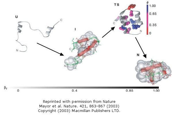
Bradley et al (2005) have taken another step forward in prediction of
tertiary structure for small proteins
(< 85 amino acids). They
describe the two biggest stumbling blocks to such predictions as the huge
number of conformations which must be explored (i.e. all of conformational
space) and accurate determination of the energy of the solvated structures.
Searching conformational space is difficult since the energy landscape
around the global energy minimum can be very steep and sharp, since
modest side chain displacements arising from subtle main chain movements
cause significant side chain packing and energy changes. The
narrowness of the energy well makes it difficult to find the global minimum
in stochastic conformational search processes. Energy calculations
also require better (more realistic) energy functions (force fields) which
show the native state to be clearly differentiated as the global minimum
from the denatured (non-native) states. They conducted energy
calculations on many different small proteins and produced for each protein
a low resolution model. To reach this low resolution model for a given
protein, they found many sequence homologs of the given target protein.
These homologs were naturally occurring sequence variants found by a
relatively conservative BLAST sequence search, with sequence identities of
30-60 percent. They also contained insertions and deletions compared
to the target sequence, which probably are involved in surface loop
structures. The target and homolog sequences were folded,
generating a more diverse population of low-resolution models as starting
points for all-atom refinement of the structure. Then, using a
new force field that stressed short range interactions (van der Waals,
H-bonding), which would expected to be more important for final folding of
the low resolution models than long range electrostatic forces), they were
able to refine the models and condense to a final low energy that was very
close in main and side chain packing to the experimental crystal structure
(resolution < 1. angstroms).
The holy grail in protein folding research has always been to predict the tertiary structure of a protein given its primary sequence. A similar but conceptually easier problem is to design a protein which will fold to a given structure with predicted secondary structure. Many possible sequences could be designed to fold to the desired structure, which makes this problem easier compared to the folding of a given sequence to just one native state. Kuhlman et al. have recently accomplished such a feat for a synthetic protein of 93 amino acids which they designed to fold to a unique topology not yet observed in nature. This represents a significant advance over earlier attempts in which mimics of known proteins were made. Such structures would be expected to fold in analogous fashions to the parent protein because of the necessary constraints placed by the need to fold to a compact state.
![]() Jmol:
Updated Top7 - A designed 93 amino acid protein with a novel
fold
Jmol14 (Java) |
JSMol (HTML5)
Jmol:
Updated Top7 - A designed 93 amino acid protein with a novel
fold
Jmol14 (Java) |
JSMol (HTML5)
Several web sites exist that allow users to download protein folding software onto their own PC. By distributing folding calculations to many home PC, their untapped computational power can be linked to provide the vast computational time needed to perform these calculations.
Additional links:
- folding of nicotine acetylcholine receptor subdomain (new 2014)
- Rosetta@home with folding Ubiquitin
- K.A. Dill, S. Banu Ozkan, T.R.Weikl, J.D. Chodera and V.A. Voelz. The protein folding problem: when will it be solved?. Current Opinion in Structural Biology 17 : 342--346 (2007). (PDF)
G6. Proteomics Problem Set 1
You will study a signal transduction protein and their interaction domains using a variety of web-based proteomics programs. For most of these programs you will need to input the amino acid sequence in FASTA format. Select a PDB code for a protein from the table at the end of this section. You could also use these programs to study any protein in the PDB.
Getting the FASTA sequence
1. First go to the PDB. Input the name
of your protein (which has an interaction domain) in the search box. Limit
the search to homo sapiens. Pick from the list of protein structure files
the most appropriate one. The example below is for the 2YYN pdb code.
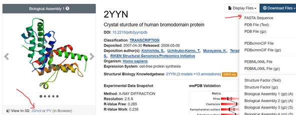
2. Select the Download Files dropdown and save the FASTA sequence to
your home directory. Download the file as a Wordpad. You might have to
remove recurring sections that don’t correspond to the single letter amino
acid sequence or identical sequences if the structure consists of identical
subunits To see if that might be the case, select JSmol (see figure above),
rotate the structure with your mouse to see if there are multiple chains,
and hover the mouse over the chains to see how the amino acids in that chain
are labeled. You might see [TRP]33A: for example, where A indicates a
separate A chain. Move to other chains. Then go to the Wordpad version of
the FASTA sequences. You can examine the chains to see if the chains are
identical. If so delete all but the first. See the above FASTA link for
help.
I. Prediction of Protein Properties from Sequence Data
Use
the following programs to gain information about your protein. Snip (with
snipping tool for example) and paste a bit of relevant info from each
program (using Snipping Tool) into this DOCX file and save it into the
folder and upload it into Sharepoint. Name the file
Lastname_LastName_FirstInitial_WebInteraction. If you have any problem with
any of the programs (lots of error messages), skip that particular program.
Several of them do the same type of analyzes. Compare the result. Snip and
paste sufficient content to show that you complete the question. Write
answers when asked to interpret the output.
a.
Sequence
Manipulation Suite: Determine the molecular weight of the protein.
b. Eukaryotic Linear Motif: Linear motifs are short, evolutionarily intrinsically
disordered section of regulatory proteins and provide low-affinity
interaction interfaces. These compact modules play central roles in
mediating every aspect of the regulatory functionality of the cell. They are
particularly prominent in mediating cell signaling, controlling protein
turnover and directing protein localization. The Eukaryotic Linear Motif
(ELM) provides the biological community with a comprehensive database of
known experimentally validated motifs, and an exploratory tool to discover
putative linear motifs in user-submitted protein sequences. Snip and paste
the top of the output that shows the IUPRED showing the disorder/order
graph.
c. TargetP
1.1 : predicts the subcellular location of eukaryotic
protein. Snip and paste the results. Interpret them based
on this link.
Where is your protein likely found?
d. NET-NES 1.1
Server:: predicts
leucine-rich nuclear export signals (NES) in eukaryotic protein This link
will help you
explain
the output. Does yours?
e. NLSdb --
Database of nuclear localization signals: Search for information on nuclear localization
signals (NLSs) and nuclear proteins. Select Query. Input the PDB code and
select NL. Does yours?
f. NetPhos
2.0 server: produces neural network
predictions for serine, threonine and tyrosine phosphorylation sites in
eukaryotic proteins. (other cool prediction programs from this site)
g.
TMPRED: The TMpred program makes a prediction of membrane-spanning regions
and their orientation. The algorithm is based on the statistical analysis of
TMbase, a database of naturally occurring transmembrane proteins. The
prediction is made using a combination of several weight-matrices for
scoring. Paste in your FASTA sequence but remove the header before running.
Does it have a transmembrane helix?
h.
TopPred 1.1 – Topology predictor
for membrane proteins at the Pasteur Institute. You will have to input your
email address. Paste in the entire FASTA file. Does it have transmembrane
helices? (Part of
Mobyle)
Save the first graph (PNG graphic file) of the
output, open it with Adobe Photoshop, and paste the image into your report.
Does the graph show alternating hydrophobic (+ values)/hydrophilic (-
values) sections consistent with transmembrane helices (for example you
would expect to see 7 hydrophobic stretches for GPCR)?
i. PFAM –
multiple analyses of Protein FAMilies. This program looks at the domain
organization of a protein sequence. Input the pdb code. When finished,
select “sequences” in the list below.

Then select the human sequence. Snip the resulting diagram and legend
showing the domain structure of the protein. You can also click on each
domain in the diagram to get more info on the domain. Does the protein have
the domain suggested in the beginning table?
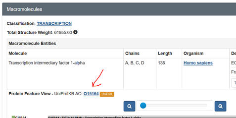
j. Prosite: Input your
FASTA sequence in the Quick Scan mode. Select Exclude motifs with a high
probability of occurrence from the scan. Snip and Paste the Hits by Proifle
domain structure. Sometimes you might need a different code number, the
UniProtKB: Accession number. Get this from the PDB web page as shown below:
k.
eFindSite: is a ligand binding site prediction and virtual screening
algorithm that detects common ligand binding sites. Put in the PDB code and
then the pdb file you downloaded.
l.
eFindSitePPI: detects protein
binding sites and residues using meta-threading. It also predicts
interfacial geometry and specific interactions stabilizing protein-protein
complexes, such as hydrogen bonds, salt bridges, aromatic and hydrophobic
interactions
m.
NCBI Standard Protein BLAST: Input the FASTA file. The
output shows the domain and domain superfamily followed by other protein
sequences nearly identical to your protein. The results are graphical
followed by descriptive. Snip domain structure with the closest aligned
sequences. Then select under PDB structures the pdb code (example below
1xww).
You will see a window similar to below. Select under domain
1xwwwA00 (as an example). :
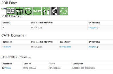
Then select the UniProtKB accession number. Confirm the many of the
predictions you made above.
n. Predict
Protein Open: Physiochemical properties of your protein.
You will have to provide your email address. When complete you can access
much of what you learned above by the links to the left under the Dashboard.
II. Visualizing Protein Interactions
It is important to be able to visualize the binding interactions between the targeted domain and the ligand (small molecule, PTM modified protein, protein or DNA). Here are some programs that allow that. Note: which programa you select will depend on if your protein is bound to a small ligand or to another protein or other macromolecule, in which case you need to explore protein interaction interfaces.
LIGAND:PROTEIN INTERACTIONS
Assignment: You will study the interaction of Protein Kinase C (PKC) with
the ligand phorbal ester, which is a mimic of the 2nd messenger
diacylglyceride with two programs: Ligand Explorer and Protein-Ligand
Interaction Profilers
a. Ligand Explorer is a Java-based program. It probably will NOT work
on a Mac running Safari. You will need the latest version of Java to run it.
Try the various computer labs around campus as well. Go to the PDB page for
your protein. After you input the pdb code, scroll down to Small Molecules
section in the middle of the displayed page for that complex. There are
links for both 2D and 3D visualization of the interactions. .
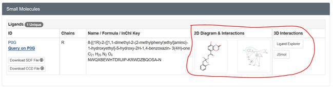
Select the 2D plot showing the interactions. The select Jsmol to see the
ligand with a binding surface) interacting with contact residues in the
protein. You can select a white background and toggle on and off H bonds.
SNIP and PASTE.
Now select Ligand Explorer for a more detailed view. Make
sure to select the correct ligand (see table below). You may be prompted to
allow pop-ups form the site. If so, allow it. You may have to reselect
Ligand Explorer again to start the program. Keep giving permissions and
following prompts until Ligand Explorer is open. Once launched, select open
this link in a new tab or window and instructions will open in a browser.
Use the mouse to help find the best view of the interactions.
Select in
turn hydrogen bond, hydrophobic, bridged H bond (mediated by a water
molecule) and metal interaction (shown on the left hand side. Select Label
Interactions by Distance. Take a cropped screenshot of each interaction (see
instructions below).
For the final rendering, move the toggle on the
Select Surfaces to opaque. Then change the distance in the best way to show
the cavity in which the ligand binds. Color by hydrophobicity which gives
two colors representing nonpolar and polar parts of cavity. Select solid
surfaces
b.
Protein-Ligand Interaction Profilers: Input the name of
your PDB file. After the run is complete, select SMALL MOLECULE and then the
appropriate ligand. You will get a 2D representation you can snip and paste.
Then select Pymol 3D view (first 5 computers in ASC 135). You will see an
interactive rendering of a small bound ligand and the protein residues it
contacts in the complex. You can get a
free student download of Pymol for
your own computer. Snip and Paste relevant info.
PROTEIN:MACROMOLECULE SURFACE INTERACTIONS
You will study
protein:protein interactions between a Src domain and small phospho-Tyr
peptide using InterProSurf and COCOMAPS.
a. InterProSurf: Reports numbers of surface and buried atoms for each chain, and areas for each residue deemed to be in the interface. Select PDB Complex in the top menu tabs and input your pdb file. This gives numerical data only. Snip and Paste relevant info.
b.
COCOMAPS: analyzes and visualizes interfaces in biological complexes
(such as protein-protein, protein-DNA and protein-RNA complexes). Input the
PDB file name and then the chains within the PDB file that you wish to see
the interaction surface. Put in the letter for one of the interacting chains
you selected into the first input box and the second letter into the second
box. Detailed results will appear in graphical and tabular form.
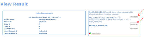
A great way to visualize the binding interface is to download the new .pdb and .pml files and open the pdb file in Pymol . Once the PDB file is opened in Pymol, select file -> run -> script_name.pml. Snip and Paste relevant info.
Table: Signaling Proteins for Analysis
|
Domains in Signaling Molecules |
||||
|
Domain |
Binding Target |
Cellular Process |
Example protein |
Pdb file |
|
Bromo |
Acetyl-Lys |
Chromatin reg. |
BRD4 |
2YYN |
|
C1 |
diacylglycerol |
Plasma memb recruitment |
Raf-1 |
3OMV |
|
C2 |
Phospholipid (Ca dependent) |
Membrane targeting, vesicle trafficking |
PRKCA |
3IW4 |
|
CARD |
Homotypic interactins |
apoptosis |
CRADD |
3CRD |
|
Chromo |
Methyl-Lys |
Chromo reg, gene txn |
CBX1 |
3F2U |
|
Death (DD) |
Homotypic inter. |
Apoptosis |
Fas |
3EZQ |
|
DED |
Homotypic inter. |
Apoptosis |
Caspase 8 |
1F9E |
|
DEP |
Memb, GPCRs |
Sig trans, prot trafficking |
Dsh human dishevelled 2 |
2REY |
|
GRIP |
Arf/Art G prot |
Golgi traffic |
Golgin-97 (Golga5) |
1R4A |
|
PDZ |
C-term peptide motifs |
Diverse, scaffolding |
PSD-95 Or discs large homolog 4 |
1L6O |
|
PH |
Phospholipids |
Membrane recuirt |
Akt |
1O6L 3CQW |
|
PTB |
Phosphor-Y |
Y kinase signaling |
Shc 1 SHC-transforming protein 1 |
1UEF 1irs europe |
|
RGS |
GTP binding pocket of Galpha |
Sig trans |
RGS4 |
1EZT |
|
SH2 |
phosphoY |
pY-signaling |
Src |
4U5W |
|
SH3 |
Pro-rich sequence |
Diverse, cytoskelet |
Src |
2PTK |
|
TIR |
Homo/Heterotypic |
Cytokine and immune |
TLR4 |
3VQ2 |
|
TRAF |
TNF signaling |
Cell survival |
TRAF-1 |
3ZJB |
|
VHL |
hydroxyPro |
ubiquitinylation |
VHL |
1VCB |
|
|
|
|
|
|
|
Protein Ligand and Protein Protein Interactions |
||||
|
Protein (PKC) :Ligand (phorbal ester mimic of 2nd
messenger diacylglyceride with Ligand Explorer and |
1PTR |
|||
|
Protein (Chain E-Src fragment) : Protein (Chain I –
phospho-peptide) with
COCOMAPS |
1QG1 |
|||
|
H-Ras-GppNHp bound to the Ras binding domain (RBD) of Raf
Kinase GppNHp binding with Ligand Explorer and
Protein-Ligand Interaction Profilers Protein (Ras, chain A):Protein (RBD-Raf, Chain B)
interactions with
COCOMAPS |
4G0N |
|||
G7. Proteomics Problem Set 2
You will study a protein, Myelin Regulatory Factor (MYRF), which
may be a transcription factor. One way to learn more about the features and
likely function of the MYRF protein is to explore the structure of the 1,139
amino acid sequence in silico.
You will analyze the protein sequence using a variety of web-based
proteomics programs. For most of these programs you will need to input
the amino acid sequence in FASTA format. Here is the
FASTA amino acid
sequence (in single letter amino acid code).
Use these programs to gain information about this protein. If
you have any problem with any of the programs (lots of error messages), skip
that particular program.
a.
Sequence
Manipulation Suite: Determine the molecular weight of the
protein.
b.
Eukaryotic Linear Motif
: Linear motifs are short, evolutionarily
plastic components of regulatory proteins and provide
low-affinity interaction interfaces. These compact modules play central
roles in mediating every aspect of the regulatory functionality of the cell.
They are particularly prominent in mediating cell signaling, controlling
protein turnover and directing protein localization. Given their importance,
our understanding of motifs is surprisingly limited, largely as a result of
the difficulty of discovery, both experimentally and computationally. The
Eukaryotic Linear Motif (ELM) provides the biological community with a
comprehensive database of known experimentally validated motifs, and an
exploratory tool to discover putative linear motifs in user-submitted
protein sequences.
c.
PSORT II:
programs for prediction of eukaryotic sequence subcellular localization as
well as other datasets and resources relevant to cellular localization
prediction. After running it, examine the link shown as PSORT features and
traditional PSORTII prediction.
You might get an error message saying the
protein does not begin with an N (Met). Met is the first amino
acid encoded from a gene sequence in eukaryotes (using the codon AUG).
It is usually removed after or during protein synthesis. Don’t’ worry
about it. Either way, the output shows you the number of homologous
proteins found and where they are located (cyto, nuc, secreted, etc). Go to
the Details link and the protein are listed. The ones on top are most
homologous to the MYRF.
d. NucPred:
analyses a eukaryotic protein sequence and predicts if the protein spends at
least some time in the nucleus or spends no time in the nucleus
f.
CCTOP -
Prediction of transmembrane helices and topology of proteins. Select
the advanced tab. This program might not work. In the
output under each amino acid you will see I (inside), O (outside), H for
transmembrane helical region, and i of indeterminate.
g.
Das-TMfilter:
might have to remove nonsequence part of fasta file
h.
TopPred 1.1 – Topoloyg predictor for membrane proteins at
the Pasteur Institute. You will have to input your email address.
http://bioweb.pasteur.fr/seqanal/interfaces/toppred.html
i.
PFAM
– multiple analyses of Protein FAMilies. View a sequence. Look
at the domain organization of a protein sequence. Input MRF_Mouse.
Click on the various domains discovered based on sequence homology.
j.
Prosite:
input your sequence in the fast scan region.
Prosite can
determine the likely function of the protein MYRF based on presence of
"patterns, motifs, or signatures " in the protein sequences which are
characteristic of a specific biological function, such as ligand binding,
catalysis, in vivo chemical modification. We will only use it to probe
for post-translational modification sites. Select Scan a
sequence against PROSITE patterns and profiles, and see possible sites
for in vivo chemical modification of the protein. In Prosite Tools uncheck
exclude patterns of high probability of occurrence.
k.
HHPRED will give you homology detection and structure
prediction, returning domain information and alignment with other proteins
of known function. Select the input link (FASTA format) to input your
sequence.
l.
NCBI Standard Protein BLAST:
m. m.
Use CATH
(Protein Structure Classification - Class, Architecture, Topology,
homology Superfamilies) to determine its domain structure and the
superfamily it resides in. Select Search and type in 1XWW in the
ID/Key Word box. Select return. Determine its class,
architecture, topology and homologous Superfamily classifications.
After search, select the BLAST tab, then select CATH Code OR click CATH Code
Superfamily (whichever works)Go to
n.n.
UniProt and input
the mouse MYRF sequence (accession number Q3UR85)for a trove of information
which you have probably just discovered.
G8. General Links and References
- Bradley, P. et al. Toward high-resolution de novo structure prediction for small proteins. Science. 309, 1868 (2005)
- Boyle J. A. Bioinformatics in Undergraduate Education. Biochemistry and Molecular Biology Education. 32, 236 (2004)
- Feig, A. L., & Jabri, E. . Incorporation of Bioinformatics Exercises into the Undergraduate Biochemistry. Biochemistry and Molecular Biology Education. 30, 224 (2002)
- Mayor et al. The complete folding pathway of a protein from nanoseconds to microseconds. Nature 421, pg 863 (2003)
- Zhou and Karplus. Interpreting the folding kinetics of helical proteins. Nature 401, pg 400(1999)

Biochemistry Online by Henry Jakubowski is licensed under a Creative Commons Attribution-NonCommercial 4.0 International License.