Biochemistry Online: An Approach Based on Chemical Logic
CHAPTER 5 - BINDING
A: INTRODUCTION TO REVERSIBLE BINDING
BIOCHEMISTRY - DR. JAKUBOWSKI
Last Update: 3/25/16
|
Learning Goals/Objectives for Chapter 5A: After class and this reading, students will be able to
|
We have studied macromolecule structure. Now it is time to impart function to these molecules. It is simple to imagine that before these molecules can perform a function, they must interact with specific molecule(s) or ligand(s) in their environment. In fact, binding and subsequent release of a ligand might be the sole function of the macromolecule (example myoglobin binding oxygen). Binding is the first step necessary for a biological response (with the exception of visual transduction in which photo-induced isomerization of rhodopsin initiates the response). To understand binding, we must consider the equilbria involved, how binding is affected by ligand and macromolecule concentrations, and how to experimentally analyze and produce binding curves.
A1. Reversible Binding of a Ligand to a Macromolecule
These derivations can be made and interpreted
using simple principles from General Chemistry, which you reviewed and
strengthened in Analytical Chemistry, with some slight differences.
Biochemists rarely talk about equilibrium or association constants, but
rather their reciprocals - the dissociation constants, Kd. For
the reactions M + L <====> ML, where M is free macromolecule, L is free
ligand, and ML is macromolecule-ligand complex (which is held together by
intermolecular forces, not covalent forces), the Kd is given by
[M]eq[L]eq/[ML]eq.
Figure: M is free macromolecule, L is free ligand, and ML is macromolecule-ligand complex
Notice the unit of Kd is molarity, M. The lower the Kd (i.e. the higher the [ML] at any given M and L), the tighter the binding. The higher the Kd, the looser the binding. Kd's for biological molecules are finely tuned to their environments. They vary from about 1 mM (weak interactions) for some enzyme-substrate complex, to pM - fM levels. Examples of very tight, non-covalent interactions include the avidin (an egg protein)-biotin (a vitamin) and thrombin (enzyme initiating clotting)-hirudin (a leech salivary protein) complexes.
M = macromolecule; L = ligand
For a simple equilibrium M + L <--> ML
where M = free macromolecule, L = free ligand, and ML = bound M and L (a complex)
3 equations can be written:
Equation 1 - Dissociation constant: K d = ([M]eq[L]eq)/[ML]eq = ([M][L])/[ML] (units of molarity)
Equation 2 - Mass Balance of M: Mo = M + ML
Equation 3 - Mass Balance of L: Lo = L + ML
We would like to derive equations which give ML as a function of known or measurable values. The Kd equations shows that ML depends on free M and free L. From Equations 1-3, two different and equally valid equations can be derived for two different cases.
- Case 1: used either when you can readily measure free L or when experimental conditions are such the Lo >> Mo, which is often encountered. Under these latter conditions, free L = Lo, which you know without measuring it, simply by knowing how much total ligand was added to the system.
- Case 2 (more general): used when you don't know free L or haven't measured it, and you just wish to calculate how much ML is present at equilibrium. These conditions imply that Lo is not >> Mo. (If Lo >> Mo, we would know free L = Lo.)
EXPERIMENTAL CASE 1: USE THIS FORM OF THE EQUATION WHEN L IS MEASURABLE OR WHEN Lo >> Mo (i.e. L= Lo)
Equation 4 - Substitute 2 into 1: K d = ([M][L])/[ML] = [Mo-ML][L])/[ML]
(ML)Kd = (Mo)L - (ML)L
(ML)Kd + (ML)L = (Mo)L
(ML)(Kd+L) = (Mo)L
Equation 5: ML = MoL/(Kd + L)
This equation is ALWAYS TRUE for the chemical equation written above. L is the free ligand concentration at equilibrium. If Lo >> Mo, then the equations simplifies to:
Equation 6: ML = MoLo/(Kd + L), whose graph you should draw below.
Dividing Equation 5 by Mo gives the fractional saturation of the macromolecule M, where
Equation 7: Y = θ= [ML]/Mo = L/(Kd + L)
where Y can vary from 0 (when L = 0) to 1 (when L >> Kd)
Graphs of ML vs L (equation 5) and ML vs Lo
(equation 6), when Lo >> Mo, and Y vs L (equation 7) are all HYPERBOLAs
Equations 5. ML = MoL/(Kd + L) (and by analogy 6 and 7) can be understood best by examining three cases:
Case 1: L = 0, ML = 0
Case 2: L = Kd, ML = MoL/(L + L)= MoL/2L = Mo/2
which indicates that M is half saturated. In fact the operational definition of Kd is the ligand concentration at which the M is half saturated.
Case 3: L >> Kd, ML = Mo
EXPERIMENTAL CASE 2 (more general): USE THIS FORM OF THE EQUATION WHEN FREE L IS NOT KNOWN (such as when Lo is not >> Mo) OR YOU WISH TO CALCULATE ML FROM JUST Lo, Mo AND KD
Equation 8 - Substitute 2 AND 3 into 1: K d = ([M][L])/[ML] = [Mo-ML][Lo-ML]/[ML]
(ML)Kd = (Mo - ML)(Lo - ML)
(ML)Kd = (Mo)(Lo) - (ML)(Lo) - (ML)(Mo) + (ML)2 or
Equation 9: (ML)2 - (Lo + Mo +Kd)(ML) + (Mo)(Lo) = 0, which is of the form
ax2 + bx + c = 0, where
-
a = 1
-
b = - (Lo + Mo +Kd)
-
c = (Mo)(Lo)
which are all constants, and
x = {-b +/- (b2 - 4ac)1/2}/2a or
Equation 10: ML = {(Lo+Mo+Kd) - ((Lo+Mo+Kd)2 - 4MoLo)1/2}/2
A graph of ML calculated from this formula vs free L (or Lo if Lo >> Mo) give a A HYPERBOLA
In the derivations, we came up with two equations for ML:- one (Equation 5) using mass conservation on M, which gave: ML = MoL/[Kd +L]
- one (Equation 10) using mass conservation on M and L, which gave ML = quadratic equation as function of Mo, Lo, and Kd: ML = {-(Lo+Mo+Kd) +/- ((Lo+Mo+Kd)2 - 4MoLo)1/2}/2
Both equations are valid. In the first you must known free L which is often Lo if Mo << Lo. In the second, you don't need to know free M or L at all. At a given Lo, Mo, and Kd, you can calculate ML, which should be the same ML you get from the first equation if you know free L.
Equations 5 and 10 are useful in several circumstances. They can be used to
- calculate the concentration of ML if Kd, Mo, and L (for equation 5) or if Kd, Mo, and Lo (for equation 10) are known. This is analogous to the use of the Henderson-Hasselbach equation to calculate the protonation state (HA) and hence charge state of an acid at various pH values. In the former case we are measuring the concentration of bound ligand (ML) and in the later case, the concentration of bound protons (HA).
- calculate Kd if ML, Mo, and L (for equation 5) or if ML, Mo, and Lo (for equation 10) are known. Techniques to extract the Kd from binding data will be discussed in the next chapter section.
A2. Interpretation of Binding Analyzes
It is important to get a mathematical understanding of the binding equations and graphs. It is equally important to get an intuitive understanding of their properties. Just as we used the +/- 2 rule in determining at a glance the charge state of an acid, you need to be able to determine the extent of binding (how much of M is bound with L) given their relative concentrations and the Kd. The usual situation is that [Mo] is << [Lo]. What happens to the binding curves for M + L <===> ML if the Kd gets progressively lower? Intuitively, you should expect that binding will increase, especially as L gets greater. The curves below should help you develop the intuition you need with respect to binding equilibria.
Fig: ML vs L at Even Lower Kd's
Fig: ML vs L at a Very Low Kd!
Note that in the last graph, given the same Mo and Lo concentrations, the "titration curves" for a binding equilibrium characterized by even tighter binding (for example, a Kd = 0.5 pM or 0.05 pM) would be indistinguishable from the graph when Kd = 5 pM. It should be apparent that for all of these Kd values, all of the added ligand is bound until [Lo] > [Mo]. To differentiate these cases, much lower ligand concentrations would be required such that on addition of ligand, all is not bound. Also note that this curve is NOT hyperbolic, which makes sense since the graph is of Y vs Lo, not Y vs L, and since Lo is not >> Mo.
![]() Wolfram
Mathematica CDF Player - Interactive Graph of Y vs L at different Kd values
(free plugin required)
Wolfram
Mathematica CDF Player - Interactive Graph of Y vs L at different Kd values
(free plugin required)
It is quite interesting to compare graphs of Y (fractional saturation) vs L (free) and Y vs Lo (total L) in the special case when Lo is not >> Mo. Examples are shown below when Mo = 4 μM, Kd = 0.19 μM . Under the ligand concentration used, it should be apparent the L can't be approximated by Lo.
Figure: Y vs L and Y vs Lo when Lo is not >> Mo
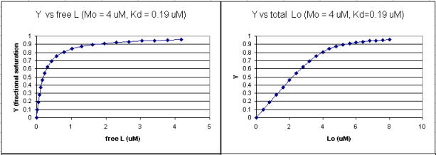
Two points should be evident from these graphs when L is not approximated by Lo:
-
a graph of Y vs Lo is not truly hyperbolic, but it does saturate
-
a Kd value (ligand concentration at half-maximal binding) can not be estimated by inspection from the Y vs Lo, but it can be from the Y vs L graph.
Fig: Comparison of Covalent Binding of Protons vs Noncovalent Binding of Ligand
A3. Dimerization and Multiple Binding Sites
In the previous examples, we considered the case of a macromolecule M binding a ligand L at a single site, as described in the equation below:
M + L <==> ML
where Kd = [M][L]/[ML]
We saw that the binding curves (ML vs L or Y vs L are hyperbolic, with a Kd = L at half maximal binding.
A special, yet common example of this equilibrium occurs when a macromolecule binds itself to form a dimer, as shown below:
M + M <==> M2 or D
where D is the dimer, and where
Equation 11: Kd = [M][M]/[D] = [M]2/[D]
At first glance you would expect a graph of [D] vs [M] to be hyperbolic, with the Kd again equaling the [M] at half-maximal dimer concentration. This turns out to be true, but a simple derivation is in order since in the previous derivation, it was assumed that Mo was fixed and Lo varied. In the case of dimer formation, Mo, which superficially represents both M and L in the earlier derived expression, are both changing.
One again a mass balance expression for Mo can be written:
Equation 12: [Mo] = [M] + 2[D]
where the coefficient 2 is necessary since their are 2 M in each dimer.
More generally, for the case of formation of trimers (Tri), tetramers (Tetra), and other oligomers,
Equation 13: [Mo] = [M] + 2[D] + 3[Tri] + 4[Tetra] + ....
Rearranging (12) and solving for M gives
Equation 14: [M] = [Mo] -2[D]
Substituting (14) into the Kd expression (1) gives
Kd = (Mo-2D)(Mo-2D)/D where can be rearranged into quadratic form:
Equation 15: 4D2 - (4Mo+Kd)D + (Mo)2 = 0
which is of the form y = ax2+bx+c. Solving the quadratic equation gives [D] at any given [Mo]. A value Y, similar to fractional saturation, can be calculated, where Y is the fraction of total possible D, which can vary from 0-1.
Equation 16: Y = 2[D]/[Mo].
A graph of Y vs Mo with a dimerization dissociation constant Kd = 25 uM, is shown below.
Figure: Saturation binding curve for dimerization of a macromolecule
Note that the curve appears hyperbolic with half-maximal dimer formation occurring at a total M concentration Mo = Kd. Also note, however, that even at Mo = 1000 uM, which is 40x Kd, only 90% of the total possible D is formed (Y = 0.90). For the simple M + L <=> ML equilibrium, if Lo = 40x the Kd and Mo << Lo,
Y = L/(Kd+L) = L/[(L/40)+L] = 0.976
The aggregation state of a protein monomer is closely linked with its biological activity. For proteins that can form dimers, some are active in the monomeric state, while others are active as a dimer. High concentrations, such as found under conditions when protein are crystallized for x-ray structure analysis, can drive proteins into the dimeric state, which may lead to the false conclusion that the active protein is a dimer. Determination of the actual physiological concentration of [Mo] and Kd gives investigators knowledge of the Y value which can be correlated with biological activity. For example, interleukin 8, a chemokine which binds certain immune cells, exists as a dimer in x-ray and NMR structural determinations, but as a monomer at physiological concentrations. Hence the monomer, not the dimer, binds its receptors on immune cells. Viral proteases (herpes viral protease, HIV protease) are active in dimeric form, in which the active site is formed at the dimer interface.
Another Special Case: Binding of L to 2 sites with different Kds
Check out the interactive graph to see how the relative sizes of the Kds affect it.
![]() Wolfram
Mathematica CDF Player - Binding of L to 2 Sites (free
plugin required)
Wolfram
Mathematica CDF Player - Binding of L to 2 Sites (free
plugin required)
A4. The Binding Continuum
Binding affinities give us a way to measure the relative strength of binding between two substances. But how "tight" is tight binding? Weak binding? Let us exam that issue by considering a binding continuum. Consider two substances, A and B that might interact. Over what range of strengths can they actually bind to each other? It would helpful to set up the extremes of the binding continuum. At one end is no binding at all. At the other end, consider two things that bind covalently. We have discussed how Kd reflects binding strength. Remember, Kd = 1/Keq. Also, we know that Keq is related to ΔGo, by the equations: ΔG o = - R T ln Keq = RT ln Kd. Given these simple equations, you should be able to interconvert between Keq, Kd, and ΔG o. (Keep your units straight.).
NO INTERACTION: One end of the binding continuum represents no interaction. Let's assume that Keq is tiny (Kd large), for example Keq ~ 2.4 10-72. Plugging this into the equation ΔG o = - R T ln Keq, where R = 2.00 cal/mol.K, and T is about 300K, the ΔGo ~ +100 kcal/mol. That is, if we add A + B, there is no drive to form AB. If AB did form, then it would immediately fall apart.
COVALENT INTERACTION: At the other end of the continuum consider the interaction of 1H atom with another to form H2. From a general chemistry book we can get ΔGoform. Using General Chem. thermodynamics, we can calculate ΔGo for H-H formation. (ΔGo = ΣGoform prod. - ΣGoform react.) Doing this gives a value of -97 kcal/mol.
SPECIFIC AND NONSPECIFIC BINDING: Consider the interaction of a protein, the lambda repressor (R), with a small oligonucleotide to which it binds tightly (called the operator DNA, O). This is an example of a biologically tight, but reversible interaction. R can bind to many short oligonucleotides due to electrostatic interactions and H bonds from the positively charged protein to the negatively charge nucleic acid backbone. The tight binding interaction, however, involves oligonucleotides of specific base sequence. Hence we can distinguish between tight binding, which usually involves specific DNA sequence and weak binding which involves nonspecific sequences. Likewise, we will speak of specific and nonspecific binding. R and O, which bind with a Kd of 1 pM, is an example of specific binding, while R and nonspecific DNA (D), which bind mostly through electrostatic interactions with a Kd of 1 mM, is an example of nonspecific binding. You might expect any positively charged protein, like mitochondrial cytochrome C, would bind negatively charged DNA. This nonspecific interaction would have no biological significance since the two are localized in different compartments of the cell. In contrast, the interaction between positively charged histone proteins, bound to DNA in the nucleus, would be specific.
RATE CONSTANTS FOR ASSOCIATION AND DISSOCIATION: When the reaction
M +
L <-===> ML is at equilibrium, the rate of the forward reaction is equal to
the rate of the reverse reaction. From General Chemistry, the forward
reaction is biomolecular and second order. Hence the vf, the rate in the
forward direction is proportional to [M][L], or
vf = kf [M][L], where kf
is the rate constant in the forward direction. The rate of the reverse
reaction, vr is first order, proportional to [ML], and is given by vr = kr
[ML], where kr is the rate constant for the reverse reaction. Notice that
the units of kf are M-1s-1, while units of kr are s-1. At equilibrium, vf =
vr, or kf [M][L] = kr [ML]. Rearranging the equation gives [ML]/[M][L]= kf/
kr = Keq. Hence Keq is given by the ratio of rate constants. For tight
binding interactions, Keq >> 1, Kd << 1, and kf is very large (in the order
of 108-9 ) and kr must be very small (10-2 - 10 -4 s-1).
To get a more intuitive understanding of Kd's, it is often easier to think about the rate constants which contribute to binding and dissociation. Let us assume that kr is the rate constant which describes the dissociation reaction. It is often times called koff. It can be shown mathematically that the rate at which two simple object associate depends on their radius and effective molecular weight. The maximal rate at which they will associate is the maximal rate at which diffusion will lead them together. Let us assume that the rate at which M and L associate is diffusion limited. The theoretical kon is about 108 M-1s-1. Knowing this, the Kd and the fact that kon/ koff = Keq = 1/Kd, we can calculate koff, which remember is a first order rate constant..
We can also determine k off experimentally. Imagine the following example. Adjust the concentrations of M and L such that Mo << Lo and Lo>> Kd. Under these conditions of ligand excess, M is entirely in the bound from, ML. Now at t = 0, dilute the solution so that Lo << Kd. The only process that will occur here is dissociation, since negligible association can occur given the new condition. If you can measure the biological activity of ML, then you could measure the rate of disappearance of ML with time, and get koff. Alternatively, if you could measure the biological activity of M, the rate at which activity returns will give you koff.
Now you will remember from General Chemistry that from a first order rate constant, the half-life of the reaction can be calculated by the expression: k = 0.693/t1/2. Hence given koff, you can determine the t1/2 for the associated species existence. That is, how long will a complex of ML last before it dissociates? Given ΔGo or Kd, and assuming a kon (108 M-1s-1 ), you should be able to calculate koff and t1/2. Or, you could be able to determine koff experimentally, and then calculate t1/2. Applying these principles, you can calculate the parameters below.
Calculated koff and t1/2 for binary complexes assuming diffusion-controlled kon
|
Complex |
KD (M) |
koff (s-1) |
t ½ |
|
H2 |
1 x 10-71 |
1 x 10-63 |
2 x 1055 yr |
|
RtV3 : Rt'L3(a) |
10-17 |
1 x 10⁻⁹ |
2 yr |
|
Avidin:biotin |
10-15 |
1 x 10⁻⁷ |
80 days |
|
thrombin:hirudin(b) |
5 x10-14 |
5 x 10⁻⁶ |
2 days |
|
lacrep:DNAoper(c) |
1 x 10-13 |
1 x 10⁻⁵ |
0.8 days |
|
Zif268:DNA(d) |
10-11 |
1 x 10⁻³ |
700 s |
|
GroEL:r-lactalbumin(e) |
10-9 |
0.1 |
7 s |
|
TBP:TATA(f) |
2 x 10⁻⁹ |
2 x 10⁻¹ |
3 s |
|
TBP:TBP |
4 x 10⁻⁹ |
4 x 10⁻¹ |
2 s |
|
LDH (pig): NADH(g) |
7.1 x 10⁻⁷(j) |
7.1 x 101 |
10 ms |
|
profilin: CaATP-G-actin |
1.2 x 10⁻⁶ |
1.2 x 10² |
6 ms |
|
TBP: DNAnonspec(h) |
5 x 10⁻⁶ |
5 x 10² |
1 ms |
|
TCR(i): cyto C peptide |
7X10⁻⁵ |
7X10³ |
100 us |
|
lacrep:DNAnonspec(h) |
1 x 10⁻⁴ |
1 X10⁴ |
70 us |
|
uridine-3P: RNase |
1.4 x 10⁻⁴ (j) |
1.4X10⁻⁴ |
50 us |
|
Creatine Kinase: ADP |
8.2 x 10⁻⁴ (j) |
8.2X10⁴ |
10 us |
|
Acetylcholine:Esterase |
1.2 x 10⁻³ |
1.2 x 10⁵ |
6 us |
|
no interaction |
4 x 1073 |
4 x 1081 |
- |
-
Trivalent Vancomycin derivative RtV3 + Trivalent D-Ala-D-Ala deriv, Rt'L3'
-
Hirudin is a potent thrombin inhibitor from leach saliva
-
lac rep is the E. Coli lac operon repressor protein, and DNAoper is the specific DNA binding region in the E. Coli genome that binds to the repressor
-
Zif268 is a mouse zinc-finger binding protein
-
GroEL is a chaperone protein; r-lactalbumin is the reduced form of lactalbumin
-
TBP is the TATA Binding Protein which binds to the TATA box consensus sequence
-
LDH is lactate dehydrogenase
-
DNAnonspec is DNA which does not contain the specific DNA sequence region involved in specific
binding to a DNA binding protein -
TCR is the T-cell receptor
-
calculated from equation: KD = koff/kon.
What is usually measured is Kd and/or koff (if the koff is reasonable). This analysis is very simplified. Electrostatic forces and other orientation factors may significantly change kon, while conformational changes in the complex may prevent ready unbinding of the bound ligand, dramatically altering koff.
The structure of one of the tighest binding complexes, avidin and biotin, is shown below.
![]() Jmol:
Updated Avidin:Biotin Complex (1AVD)
Jmol14 (Java) |
JSMol (HTML5)
Jmol:
Updated Avidin:Biotin Complex (1AVD)
Jmol14 (Java) |
JSMol (HTML5)
It is important to note that even reactions characterized by high Kd can be specific. Specificity is ultimately defined as a binding interaction between a macromolecule and ligand that can be co-localized in the same environment and for which a biological function is elaborated upon binding.
A5. Experimental Analyses of Binding
It is often important to determine the Kd for a ML complex, since given that number and the concentrations of M and L in the system, we can predict if M is bound or not under physiological conditions. Again, this is important since whether M is bound or free will govern its activity. The trick in determining Kd is to determine ML and L at equilibrium. How can we differentiate free from bound ligand? The following techniques allow such a differentiation.
TECHNIQUES THAT REQUIRE SEPARATION OF BOUND FROM FREE LIGAND -
Care must be given to ensure that the equilibrium of M + L <==> ML is not shifted during the separation technique.
- gel filration chromatography - Add M to a given concentration of L. Then elute the mixture on a gel filtration column, eluting with the free ligand at the same concentration. The ML complex will elute first and can be quantitated . If you measure the free ligand coming off the column, it will be constant after the ML elutes with the exception of a single dip near where the free L would elute if the column was eluted without free L in the buffer solution. This dip represents the amount of ligand bound by M.
- membrane filtration - Add M to radiolableled L, equilibrate, and
then filter through a filter which binds M and ML. For instance, a
nitrocellulose membrane binds proteins irreversibly. Determine the amount of
radiolabeled L on the membrane which equals [ML].
- precipitation - Add a precipitating agent like ammonium sulfate,
which precipitates proteins and hence both M and ML. Determine the amount of
ML.
TECHNIQUES THAT DO NOT REQUIRE SEPARATION OF BOUND FROM FREE LIGAND
-
equilibirum dialysis - Place M in a dialysis bag and dialyze against a
solution containing a ligand whose concentration can be determined using
radioisotopic or spectroscopic techniques. At equilibrium, determine free L
by sampling the solution surrounding the bag. By mass balance, determine the
amount of bound ligand, which for a 1:1 stoichiometry gives ML. Repeat at
many different ligand concentrations
- spectroscopy - Find a ligand
whose absorbance or fluorescence spectra changes when bound to M.
Alternatively, monitor a group on M whose absorbance or fluorescence spectra
changes when bound to L.
- isothermal titration calorimetry (ITC)- In ITC, a high concentration solution of an analyte (ligand) is injected into a cell containing a solution of a binding partner (typically a macromolecule like a protein, nucleic acid, vesicle).
Figure: Isothermal Titration Calorimeter Cells
On binding, heat is either released (exothermic reaction) or adsorbed, causing a small temperature changes in the sample cell compared to the reference cells containing just a buffer solution. Sensitive thermocouples measure the temperature difference (DT1) between the sample and reference cells and apply a current to maintain the difference at a constant value. Multiple injections are made until the macromolecules is saturated with ligand. The enthalpy change is directly proportional to the amount of ligand bound at each injection so the observed signal attenuates with time. The actual enthalpy change observed must be corrected for the change in enthalpy on simple dilution of the ligand into buffer solution alone, determined in a separate experiment. The enthalpy changes observed after the macromolecule is saturated with ligand should be the same as the enthalpy of dilution of the ligand. A binding curve showing enthalpy change as a function of the molar ratio of ligand to binding partner (Lo/Mo if Lo >> Mo) is then made and mathematically analyzed to determine Kd and the stoichiometry of binding.
Figure: Typical isothermal titration calorimetry data and analysis
Reference: http://www.microcalorimetry.com/index.php?id=312
It should be clear in the example above, that the binding reaction is exothermic. But why is the graph of ΔH vs molar ratio of Lo/Mo sigmoidal (s-shaped) and not hyperbolic? One clue comes from the fact that the molar ratio of ligand (titrant) to macromolecule centers around 1 so, as explained above, when Lo is not >> Mo, the graph might not hyperbolic. The graphs below show a specific example of a Kd and ΔHo being calculated from the titration calorimetry data. They will shed light on why the graph of ΔH vs molar ratio of Lo/Mo is sigmoidal.
A specific example illustrates these ideas. Soluble versions of the HIV viral membrane protein, gp 120, 4 μM, was placed in the calorimetry cell, and a soluble form of its natural ligand, CD4, a membrane receptor protein from T helper cells, was placed a syringe and titrated into the cell (Myszka et al. 2000). Enthalpy changes/injection were determined and the data was transformed and fit to an equation which shows the ΔH "normalized to the number of moles of ligand (CH4) injected at each step". The line fit to the data in that panel is the best fit line assuming a 1:1 stoichiometry of CD4 (the "ligand") to gp 120 (the "macromolecule") and a Kd = 190 nM. Please note that the curve is sigmoidal, not hyperbolic.
Figure: Titration Calorimetry determination of Kd and DH for the interaction of gp120 and CD4
Note that the stoichiometry of binding (n), the KD, the ΔHo can be determined in a single experiment. From the value of ΔHo and KD, and the relationship ΔGo = -RTlnKeq = RTlnKD = ΔHo - TΔSo, the ΔGo and ΔSo values can be calculated. No separation of bound from free is required. Enthalpy changes on binding were calculated to be -62 kcal/mol.
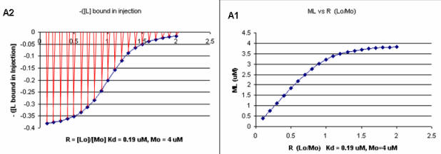
Using the standard binding equations (5, 7, and 10 above) to calculate free L and ML at a vary of Lo concentrations and R = Lo/Mo ratios, a series of plots can be derived. Two were shown earlier in this Chapter section to illustrate differences in Y vs L and Y vs Lo when Lo is not >> Mo. They are shown again below:
Figure: Y vs L and Y vs Lo when Lo is not >> Mo
Next a plot of ML vs R (= [Lo]/[Mo] (below, panel A1 right) was made. This curve appears hyperbolic but it has the same shape as the Y vs Lo graph above (right). However if the amount of ligand bound at each injection (calculated by subtracting [ML] for injection i+1 from [ML] for injection i) is plotted vs R (= [Lo]/[Mo]), a sigmoidal curve (below, panel A2, left) is seen, which resemble that best fit graph for the experimentally determine enthalpies above. The relative enthalpy change for each injection is shown in red. Note the graph in A2 actually shows the negative of the amount of ligand bound per injection, to make the graph look the that in the graph showing the actual titration calorimetry trace and fit above.
Figure: Binding Curves that Explain Sigmoidal Titration Calorimetry Data for gp120 and CD4
Surface Plasmon Resonance
A newer technique to measure binding is called surface plasmon resonance (SPR) using a sensor chip consisting of a 50 nm layer of gold on a glass surface. A carbohydrate matrix is then added to the gold surface. To the CHO matrix is attached through covalent chemistry a macromolecle which contains a binding site of a ligand. The binding site on the macromolecule must not be perturbed to any significant extent. A liquid containing the ligand is flowed over the binding surface.
The detection system consists of a light beam that passes through a prism on top of the glass layer. The light is totally reflected but another component of the wave called an evanescent wave, passes into the gold layer, where it can excite the Au electrons. If the correct wavelength and angle is chosen, a resonant wave of excited electrons (plasmon resonance) is produced at the gold surface, decreasing the total intensity of the reflected wave. The angle of the SPR is sensitive to the layers attached to the gold. Binding and dissociation of ligand is sufficient to change the SPR angle, as seen in the figure below. (Science, 295, pg 2103 (2002))
Fig: Surface Plasmon Resonance
 animation:
SPR evanaescent wave
animation:
SPR evanaescent wave
This technique can distinguish fast and slow binding/dissociation of ligands (as reflected in on and off rates) and be used to determine Kd values (through measurement of the amount of ligand bond at a given total concentration of ligand or more indirectly through determination of both kon and koff.
Binding DB: a
database of measured binding affinities, focusing chiefly on the
interactions of protein considered to be drug-targets with small,
drug-like molecules
PDBBind-CN:
a comprehensive collection of the
experimentally measured binding affinity data for all types of
biomolecular complexes deposited in the Protein Data Bank (PDB).
A6. Extreme Binding Affinities
An incredibly tight binding interaction has recently been reported for the binding of Cu1+ to the CueR protein from E. Coli. Cu1+ ions are usually kept to a very low concentration in cells as a mechanism to prevent toxicity. Yet some enzymes require Cu. Free copper ions must be present in the cell to allow binding to appropriate sites in proteins. How are these competing concerns regulated in the cell? The total Cu concentration in E. Coli is about 10 μM (10,000 nM), which, given the small size of the bacterium, represents about 10,000 copper ions per cell.
Cells have evolved many mechanisms to control and deliver Cu ions. Copper ions can be delivered to target proteins by copper chaperones (analogs of the chaperone proteins which guide protein folding). CueR in E. Coli appears to regulate the copper-induced expression of genes involved in copper biochemistry (including an enzyme that oxidizes Cu1+ to Cu2+ which is less toxic). One particular gene that is up-regulated is copA. CueR increases transcription of copA in the presence of Cu, Ag, and Au (coinage metal) ions. Changela et al. developed an in vitro assay which determined the extent of expression of CueR regulated genes, under a variety of ion types and concentrations. In the assay, purified CueR was added to a gene construct containing the promoter (a section of DNA immediately upstream of a gene start site where RNA polymerase binds) for copA. Initially they found that transcription was always on even in the presence of a ligand, glutathione, which binds Cu1+ avidly and should keep free Cu1+ levels very low. They switched to an even tighter binding Cu1+ coordinator, cyanide (CN-), to reduce the free Cu1+ levels to even lower levels. Extremely high levels of CN- (millimolar) stopped transcriptional activation, but if additional Cu1+ was added, activation ensued, suggesting that copper binding to the protein was reversible. At 1 mM CN-, transcription increased with addition of copper ions up to a TOTAL Cu1+ concentration of 60 μm. Under these condition, the free Cu1+ concentrations were much less. Given the presence of CN- concentrations used, half-maximal activation occurred at a TOTAL Cu1+ concentration of 0.7 μM. Similar activation was observed by Ag1+ and Au1+, but not by Zn and Hg ions, showing the specificity for monovalent cations over divalent cations.
Knowing the pKa of HCN, stability constants for Cu1+:CN- complexes, and CN- concentrations, Changela et al produced a series of solutions buffered in FREE Cu1+ that extended from 10-18 to 10-23 M (pH 8.0). (For example, the log of the binding constant β, logβ, for the Cu1+ + 2CN- <==> [Cu(CN)2]- is 21.7. You solved problems such as this involving linked equilibrium if you have taken analytical chemistry.) The free Cu1+ concentration at half-maximal activation of gene reporter transcription, a measure of the dissociation constant, Kd, was approximately 1 x 10-21 M (zeptomolar)! Now assume that the volume of the contents of an E. Coli cell is 1.5 x 10⁻¹⁵ L. If there were only one ion of Cu1+ in the cell, it would have a concentration of 10-9 M. The values suggest that there is no free Cu1+ ions in the cell, and that only 1 Cu+1 ion in the cell is enough to ensure its binding to CueR and subsequent transcriptional activation of copA.
![]() Jmol: Updated
Cu(I) Form Of E. Coli Cuer, A Copper Efflux Regulator
Jmol14 (Java) |
JSMol (HTML5)
Jmol: Updated
Cu(I) Form Of E. Coli Cuer, A Copper Efflux Regulator
Jmol14 (Java) |
JSMol (HTML5)
It is essential for survival that bacterial cells get the right metal to metalloproteins. A recent review by Waldron and Robinson illustrates how. The cell has many mechanisms of restricting specific binding sites so metals are able to get to the right proteins. In addition, the natural order of stability for transition metals complexes must be considered in understanding metal affinities. That stability is given by the Irving – William series which is shown below (along with Group 2A metal ions). The trend parallels the size of the cation (going from largest to smallest):
Mn2+ < Fe2+ < Co2+ < Ni2+ < Cu2+ > Zn2+ (tightest binding)
- The ability for a protein to change shape on ligand binding allows different metals to bind. For example, cyanobacterium has a high demand for copper and manganese. Manganese is allowed to bind first and then the protein is folded and manganese becomes trapped inside the protein. This very unstable metal now cannot be replaced by copper, which would ordinarily out compete Mn2+ for the site.
- Metal transporters help regulate how many ions of each metal are in the cell. Metal sensors are under the control of these metal transporters, regulating gene expression. Once a specific metal has a sufficient concentration for binding, the metal sensors target mRNA to repress certain genes and halt transcription
- Another enzyme can also be activated for the metal’s export. By restricting the concentrations of the competing metals, weaker metal-binding sites remain available
- Metal sensors can also help to regulate what protein some metals use based on what is available. For example, E. coli switches metabolism to minimize the number of iron-requiring proteins that are expressed when iron is less abundant
- Metals are supplied by multiple pathways (in case a specific enzyme is not present), and are “trafficked†to the correct protein through many ligand-exchange reactions.
- Certain enzymes bind specific metals that cause preferential conformational changes. Hence, if a metal comes along that binds more tightly but is not preferred by the enzyme, it will not trigger the enzyme because it binds in a different manner
A7. Molecular Basis of High Affinity Interactions
What differentiates high and low affinity binding at the molecular level? Do high affinity interactions have lots of intramolecular H-bonds, salt bridges, van der Waals interactions, or are hydrophobic interactions most important? Recently, the crystal structures of a variety of antibody-protein complexes were determined in order to study the basis of affinity maturation of antibody molecules. It is well know that antibodies elicited on exposure to a foreign molecule (antigen) are initially of lower affinity than antibodies released later in the immune response. An incredible number of different antibodies can be made by antibody-producing B cells due to genetic mechanisms (combining different variable regions of antibody genes through splicing, imprecise splicing, and hypermutation of critical nucleotides in the genes of antigen binding regions of antibodies). Clones of antibody-producing cells with higher affinity are selected through binding and clonal expansion of these cells. Investigators studied the crystal structure of 4 different antibodies which bound to the same site (epitope) on the protein antigen lysozyme. Increased affinity was correlated with increased buried apolar surface area and not with increased numbers of H bonds or salt bridges.
Table: Characteristics of Antibody:Hen Egg Lysozyme Complexes(HEL)
| Antibody | H26-HEL | H63-HEL | H10-HEL | H8-HEL |
| Kd (nM) | 7.14 | 3.60 | 0.313 | 0.200 |
| Intermolecular Interactions | ||||
| H bonds | 24 | 25 | 20 | 23 |
| VDW contacts | 159 | 144 | 134 | 153 |
| salt bridges | 1 | 1 | 1 | 1 |
|
Buried Surface Area |
||||
| ΔASURF (A2) | 1,812 | 1,825 | 1,824 | 1,872 |
| ΔASURF-polar (A2) | 1,149 | 1,101 | 1,075 | 1,052 |
| ΔASURF-apolar (A2) | 663 | 724 | 749 | 820 |
Li,Y. et al. Nature: Structural Biology. 6, pg 484 (2003)
Electrostatic interactions between biological molecules are still very important interactions, even though we may consider them to be nonspecific. Witness the interaction of DNA binding proteins with positive domains with the negative polyanion, DNA. The initial encounter will be electrostatic in origin and obviously important to targeting the proteins to DNA where additional specific interactions may take place.
In a similar example (Yeung, T et al.), it was recently reported that moderately positively charged proteins are directed to endosomes and lysosomes through interactions with negatively charged membrane phosphatidylserine (PS), whereas more positively charged proteins are targeted to the inner surface of the plasma membrane, which is enriched in PS and phosphorylated phosphatidyl inositol derivatives (PIP2, PIP3), as shown below.
Figure: negatively charged phospholipids in biological membranes
To study this they used the C2 domain of lactadherin (Lact-C2) from milk that binds PS in the presence of calcium. The C2 domain was covalently linked to the green fluorescent protein, a protein which contains an internal fluorophore comprised of three amino acids (Ser65–Tyr66–Gly67) that cyclize spontaneously on folding to produce a fluorophore which emits green light. A fusion gene of Lact-C2 and GFP was introduced in wild type (WT) and mutant yeast lacking PS. It was bound to the inner leaflet in WT cells and to endosome and lysosome vesicles , but found diffused through cytoplasm in mutant cells. They also made cationic probes with farnesyl tails attached which could anchor the soluble probes to membranes. The most positively charged probes were recruited to the plasma membrane inner leaflet, while less charged ones were recruited to internal vesicles. The authors speculate that PS on cytoplasmic membrane layers can target signal transduction proteins to these regions.
Antibodies with Infinite Affinity. Chmura et al. PNAS. 98, pg 8480
(1998)
Docking
The quantitative methods described above do not elucidate the mechanism of binding. Computer programs have been developed that allow the docking of a ligand (small molecule or even another protein) to another protein. The automatic docking of flexible ligands to proteins can be modeled using Autodock. AutoDock contains the following programs:
-
AutoDock performs the docking of the ligand to a set of grids describing the target protein;
-
AutoGrid pre-calculates these grids;
-
AutoTors sets up which bonds will treated as rotatable in the ligand.
Molecular dynamics simulations can also be used to study the actual binding and unbinding processes.
The Crowded Cell
Most binding studies are performed in vitro with dilution concentrations of both macromolecule and ligand. Are these conditions illustrious of conditions inside a cell? The answer is no! Cells are very crowded with organelles, macromolecular complexes, and cytoskeletal components which provide internal architecture to the cell, etc. Total macromolecule concentration in the cell has been estimated to be as high as 400 g/1L = 400 g/1000 mL = 0.4 g/mL = 400 mg/mL. Try to dissolve a water soluble protein like albumin to those concentrations! From 5 to 40% of the entire cellular volume is occupied with large molecules, and at the upper range, very little space exists for other large macromolecules.
A8. Links and References
Waldron, K and Robinson, N. How do bacterial cells ensure that metalloproteins get the correct metal? Nat Rev Microbiol. 7, 25 (2009)
Yeung, T. et al. Membrane phosphatidylserine regulates surface charge and protein localization. Science. 319, 210-212 (2008)
Changela, A. et al. Molecular basis of metal-in selectivity and zeptomolar sensitivity by CueR. Science. 301, pg 1383 (2003)
Li, Y. et al. X-ray snapshots of the maturation of an antibody response to a protein antigen. Nature: Structural Biology, 6, pg 482 (2003)
Martin, R. B. Comparisons of Indefinite Self-Association Models. Chemical Reviews. 96, 3043 (1996).
 Navigation
Return to Biochemistry Online Table of Contents
Archived version of full Chapter 5A: Introduction to Reversible Binding

Biochemistry Online by Henry Jakubowski is licensed under a Creative Commons Attribution-NonCommercial 4.0 International License.